Module 3: SAR Fundamentals I, from Pulse to Backscatter

Phase: I, Foundations of the data, physics, and radar
Level: Intermediate
Estimated time: ~12 hours (about 6 h concepts, 5 h lab, 1 h write-up)
Prerequisites: Modules 1 and 2, Phase 0.
Portfolio thread: adds sar_prep.py and a "three RTCs, one scene" comparison plus a short public-style note, "what C-band backscatter sees after a fire." Closes Phase I.

Why this module

This is the week that separates "has used Sentinel-1" from "understands SAR." Radar is the backbone of cloud-free fire and forest monitoring, and interviewers at SAR-focused companies will ask about layover, speckle statistics, and why you terrain-corrected before they ask about your model. Optical work has an intuition most people already share; radar does not, so the payoff for building real understanding here is large and durable. It is also where careless practitioners produce confidently wrong results, by comparing uncalibrated amplitudes or ignoring terrain.

Learning outcomes

After this module you can:

1. Explain SAR imaging geometry: side-looking acquisition, slant versus ground range, and the layover, foreshortening, and shadow distortions.
2. Explain polarization (VV, VH) and the main scattering mechanisms (surface, volume, double-bounce).
3. Explain speckle: the multiplicative noise model, equivalent number of looks (ENL), multilooking, and speckle filters, and when to work in dB versus linear.
4. Define sigma-naught, gamma-naught, and beta-naught, distinguish GRD from SLC, and say what radiometric terrain correction (RTC) does.
5. Compare frequency bands (X, C, L, P) and their penetration, and explain why C-band saturates over dense forest while L-band and P-band do not.
6. Produce a terrain-corrected Sentinel-1 scene by more than one route and compare them, and ship a tested sar_prep.py.

Concept lessons (about 6 hours)

Lesson 1: Geometry, why radar images look strange

A radar is an active, side-looking sensor: it points off to the side and measures the time and strength of echoes. Because it ranges by echo travel time rather than angle, terrain creates characteristic distortions:

• Foreshortening: slopes facing the sensor are compressed, because the top and bottom of the slope return echoes close together in time.
• Layover: when a slope is steep enough that the top returns its echo before the bottom, the top appears "laid over" toward the sensor, on top of the valley.
• Shadow: terrain behind a steep slope receives no illumination and returns nothing.

Raw SAR is in slant range (echo time); you resample to ground range and, better, terrain-correct against a DEM so pixels sit in real map coordinates. This is why terrain correction is not optional in hilly terrain: without it, your backscatter is in the wrong place and the wrong brightness.

Lesson 2: Polarization and scattering

Sentinel-1 transmits and receives in polarizations, commonly VV (vertical transmit, vertical receive) and VH (vertical transmit, horizontal receive). Different surfaces scatter differently:

• Surface (single-bounce) scattering from smooth-to-rough ground shows up mostly in co-polarization (VV).
• Volume scattering from vegetation canopy (many randomly oriented scatterers) depolarizes the signal and raises cross-polarization (VH).
• Double-bounce (for example ground-to-trunk or ground-to-wall corners) is strong in co-polarization and characteristic of built structures and flooded vegetation.

Reading VV and VH together, and their ratio, is how you infer what is on the ground. After a fire, canopy volume scattering collapses, so VH usually drops; on steep terrain the picture is complicated by geometry, which is exactly the kind of nuance interviewers probe.

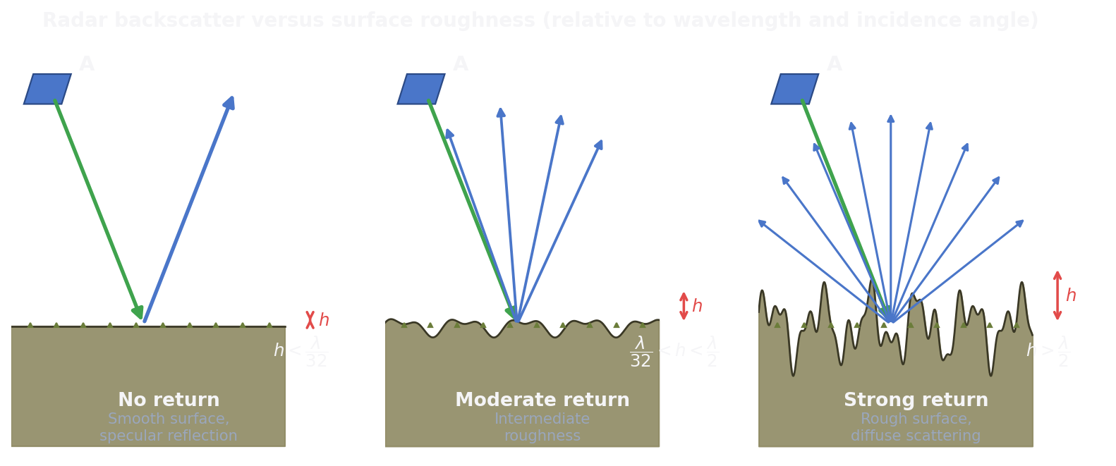
How bright a surface looks also depends on its roughness relative to the wavelength. A surface that is smooth compared to the wavelength reflects the pulse away from the sensor (specular) and returns little, so it looks dark; a rough surface scatters diffusely and sends energy back, so it looks bright. This is why calm water and paved roads are dark in Sentinel-1 while forests and built-up areas are bright.

Lesson 3: Speckle

SAR images have a grainy texture called speckle. It is not sensor noise in the usual additive sense; it is a multiplicative interference effect from coherent summation of many sub-pixel scatterers. Consequences and tools:

• Model: speckle is multiplicative, so brighter areas show larger absolute fluctuations. This is why SAR is often analyzed in decibels (a log scale) rather than linear power.
• ENL (equivalent number of looks): a measure of how much speckle has been reduced, estimated on a homogeneous patch as (mean / standard deviation) squared. Higher ENL means smoother.
• Multilooking averages independent looks to reduce speckle at the cost of spatial resolution. Speckle filters (Lee, Refined Lee, and others) reduce speckle while trying to preserve edges.
• dB versus linear: average and composite in linear power (averaging dB values is not physically meaningful), then convert to dB for display and thresholding.

Lesson 4: Radiometric terms, GRD versus SLC, and RTC

• Beta-naught, sigma-naught, gamma-naught are backscatter normalizations. Beta-naught is radar brightness; sigma-naught normalizes by the ground area; gamma-naught normalizes by the area perpendicular to the look direction and is the terrain-robust choice, which is why RTC products are usually gamma-naught.
• GRD versus SLC: Ground Range Detected products are amplitude only, multilooked, and are what you use for most backscatter and change work. Single Look Complex products keep phase and are required for interferometry and coherence (Module 9).
• RTC (radiometric terrain correction) uses a DEM to correct both the geometry and the radiometry for terrain, producing analysis-ready backscatter where a given surface has a consistent value regardless of slope. This is the required first step for amplitude-based SAR applications.

Lesson 5: Frequency bands and penetration

Radar wavelength sets what the signal interacts with:

• X-band (short): surface detail, less penetration.
• C-band (Sentinel-1): interacts with the upper canopy and roughness; it saturates over dense forest, meaning above a moderate biomass it stops responding, which limits C-band for biomass but keeps it excellent for change and structure at moderate levels.
• L-band (ALOS-2, and NISAR): longer wavelength penetrates the canopy to branches and trunks, better for forest structure and biomass; covered more in Module 9.
• P-band (ESA Biomass mission): longest, penetrates to woody biomass, purpose-built for forest carbon.

Knowing which band sees what, and why C-band saturates, is a standard interview topic and drives sensor choice in later forestry and change modules.

A note on the current constellation

Verify this at study time, because it moved recently. The Copernicus C-band radar constellation is now Sentinel-1C (launched December 2024) and Sentinel-1D (data from April 2026, fully operational May 2026). Sentinel-1A ended operations on 30 June 2026 after twelve years, and Sentinel-1B was lost earlier. In practice this means recent Sentinel-1 acquisitions come from 1C and 1D; do not assume 1A or 1B for current dates.

Guided lab (about 5 hours): one scene, three ways

You will terrain-correct one Sentinel-1 scene by three routes and compare, then build a small reusable prep module.

Step 1: Three routes to a terrain-corrected scene

Take one Sentinel-1 IW scene over your fire AOI and produce backscatter three ways:

1. ESA SNAP (the Sentinel-1 Toolbox): run the manual chain once so you understand each step: apply orbit file, thermal-noise removal, radiometric calibration, speckle filter, terrain correction (Range-Doppler against a DEM), and conversion to dB. Do it in the GUI once, then reproduce it from a saved processing graph so it is repeatable. Use the current SNAP release.
2. ASF HyP3 on-demand RTC: submit the same scene to HyP3, which returns an analysis-ready RTC product. This is the "let a service do it" route.
3. OPERA RTC-S1: fetch the matching off-the-shelf OPERA RTC-S1 tile from ASF (gamma-naught, near-global over land since 2016, delivered as COGs). This is the "already analysis-ready, no processing" route.

Reproject the three onto a common grid and compare pixel-wise: differences come from DEM choice, speckle filtering, and normalization. Write up what differs and why.

Step 2: sar_prep.py with tests

"""sar_prep.py: SAR backscatter helpers (pure, testable)."""
from __future__ import annotations
import numpy as np

def to_db(x, eps=1e-10):
    """Linear power to decibels."""
    return 10.0 * np.log10(np.maximum(x, eps))

def from_db(d):
    """Decibels to linear power."""
    return 10.0 ** (d / 10.0)

def enl(patch):
    """Equivalent number of looks on a homogeneous patch: (mean/std)^2."""
    patch = np.asarray(patch, float)
    s = patch.std()
    return float("inf") if s == 0 else float((patch.mean() / s) ** 2)

def vh_vv_ratio(vh, vv, eps=1e-10):
    """Cross- to co-pol ratio in linear power (compute before converting to dB)."""
    return vh / np.maximum(vv, eps)

def boxcar(img, size=5):
    """Simple multilook/boxcar speckle reducer (mean filter)."""
    from scipy.ndimage import uniform_filter
    return uniform_filter(np.asarray(img, float), size=size)

# tests/test_sar_prep.py
import numpy as np
from eo_portfolio.sar_prep import to_db, from_db, enl, boxcar

def test_db_roundtrip():
    x = np.array([0.5, 1.0, 2.0])
    assert np.allclose(from_db(to_db(x)), x, rtol=1e-6)

def test_to_db_known():
    assert abs(float(to_db(np.array(10.0))) - 10.0) < 1e-9

def test_speckle_filter_raises_enl():
    rng = np.random.default_rng(0)
    img = rng.gamma(shape=1.0, scale=1.0, size=(64, 64))  # exponential: speckle-like, ENL ~ 1
    assert enl(boxcar(img, 5)) > enl(img)

Remember the physical rule the tests encode: average in linear power, then go to dB; and a speckle filter should raise ENL.

Step 3: A physical time series

Build a 12-month VV and VH time series (in dB, from linear-power composites) over three cover types in your AOI: burned forest, unburned forest, and bare ground. Plot them and explain each curve physically: why unburned forest sits where it does in VH, what happens to VH after the fire, and how bare ground compares. Measure ENL on a homogeneous patch before and after your speckle filter and report it.

Step 4: Write-up and commit

A short, blog-style note: "what C-band backscatter sees after a fire," plus the "three RTCs, one scene" comparison. Commit sar_prep.py, its tests, and the notebook.

git add src/eo_portfolio/sar_prep.py tests/test_sar_prep.py notebooks/05_sar_prep.ipynb
git commit -m "Module 3: SAR prep helpers, three-RTC comparison, VV/VH time series"
git push

Checkpoint

Self-check (answers below).

1. Why must you terrain-correct Sentinel-1 before comparing backscatter across a hilly scene?
2. Why do we usually composite in linear power but display and threshold in dB?
3. What does a high ENL indicate, and how do you estimate it?
4. When would you need SLC rather than GRD products?

Interview-style questions (practice out loud).

• Why does a burned forest get darker in VH but sometimes brighter in VV, and what changes on steep terrain?
• Explain speckle to a new teammate, including why SAR is often shown in decibels.
• When would you choose C-band over L-band, and what does that imply for forest biomass?
• Walk me through turning a raw Sentinel-1 scene into analysis-ready backscatter.

Answers. (1) Terrain distorts both geometry (layover, foreshortening, shadow) and radiometry, so without RTC the same surface has different brightness on different slopes and sits in the wrong location; gamma-naught RTC removes this.
(2) Speckle and backscatter combine multiplicatively, so averaging is physically meaningful in linear power; dB is a log scale for viewing and thresholding, and averaging dB values directly is not correct.
(3) High ENL means speckle has been well suppressed (smoother image); estimate it on a homogeneous patch as (mean divided by standard deviation) squared.
(4) For interferometry and coherence, which need the phase that GRD discards; SLC preserves it.

Deliverable

A tested sar_prep.py (dB conversion, ENL, speckle filter, VH/VV ratio), a "three RTCs, one scene" comparison notebook, a 12-month VV/VH time series over three cover types with physical explanations, and a short note on what C-band sees after a fire. This closes Phase I and sets up the SAR change work in Phase II.

What a hiring manager sees

SAR is where surface-level familiarity is easy to spot and real understanding is rare. Showing that you terrain-correct deliberately, know gamma-naught from sigma-naught, handle speckle correctly (linear versus dB, ENL), and can explain a VV/VH time series physically marks you as someone a SAR team can trust with data. The three-route comparison also shows you know when to process yourself and when to use analysis-ready products, which is a practical maturity signal.

Currency note

Verified August 2026. The operational Copernicus C-band constellation is Sentinel-1C and Sentinel-1D; Sentinel-1A ended operations on 30 June 2026 and Sentinel-1B was lost earlier, so confirm which satellites cover your dates. OPERA RTC-S1 (Version 1, gamma-naught, COGs) is available from ASF in the OPERA_L2_RTC-S1_V1 collection, accessible via ASF Vertex, the asf_search package, or Earthdata Search, near-global over land since April 2016. ASF HyP3 offers on-demand RTC and InSAR from Sentinel-1 IW GRD and SLC. Use the current ESA SNAP release and verify its version and processing-operator names, since the GUI and graph steps evolve between releases. Pin all Python versions in your Module 0.1 environment file (sar_prep.boxcar uses SciPy).