Module 0.1: Your Geospatial Python Toolkit

Phase: 0, Foundations
Level: Beginner
Estimated time: 8 to 10 hours
Prerequisites: basic computer literacy, willingness to use a terminal, and the ability to read and write simple Python (variables, functions, loops, imports). No prior GIS, remote sensing, or machine learning required.
Portfolio thread: this module creates the eo-portfolio repository that every later module commits into. It is the workbench the whole course is built on.

Brand new to Python? This course uses Python from the first lab but does not teach the language from zero. If you have never written Python, spend a few hours first on a free beginner course, for example the official Python tutorial (https://docs.python.org/3/tutorial/) or Python for Everybody (https://www.py4e.com/), until you are comfortable with variables, functions, loops, lists/dicts, and imports. Then come back here.

Prefer not to install anything yet? You can run the early labs in a browser with Google Colab (https://colab.research.google.com/) or a GitHub Codespace on your eo-portfolio repo. Local setup with a committed environment file is still the goal, because reproducibility is part of what employers screen for, but a cloud notebook is a fine way to start on day one.

Where to run the labs

You do not need a powerful computer. The one-click buttons below open the eo-portfolio template, which already has the environment, tests, and a starter notebook, so you can run a lab in your browser in under a minute:

Pick whichever fits the phase:

• Phase 0 to Phase II (setup and classical ML): run locally with the environment you build below, or in the browser with GitHub Codespaces or Google Colab. No GPU needed.
• Phase III (deep learning, Modules 7 to 9): use a free GPU notebook (Google Colab or Kaggle).
• The Earth Engine step in Module 8: the Earth Engine Python API on the free noncommercial tier.
• Phase IV (Module 11): deploy to real cloud (containers and object storage); learning to do that is the point of the module.

Data is read cloud-natively from STAC catalogs (Copernicus Data Space, Microsoft Planetary Computer, NASA Earthdata), so you rarely download whole scenes wherever you compute. Start with "Use this template" once to create your own eo-portfolio repository, then use the Colab or Codespaces button on each lab.

Why this module

Open any remote-sensing or geospatial-ML job description and the same tools appear: Python, GDAL, rasterio, GeoPandas, xarray, git. Before you can learn burn severity or SAR change detection, you need a workbench where you can install these tools, run code reproducibly, and show your work in version control. Employers do not just want a notebook that ran once on your laptop. They want a repository with an environment, tests, and continuous integration, because that is how real teams work. We build that first, so from Module 1 onward you are adding science to a professional foundation rather than fighting your setup.

Learning outcomes

After this module you can:

1. Create a reproducible Python environment and explain why reproducibility matters.
2. Use git and GitHub to version your work and push it publicly.
3. Read, slice, and plot arrays and tables with numpy, pandas, and matplotlib.
4. Name the core geospatial libraries, say what each one does, and describe how they fit together.
5. Open a raster and a vector file in Python, inspect their metadata, and plot them.
6. Ship all of the above as a tested repository with green continuous integration.

Concept lessons (about 3 hours)

Lesson 1: The reproducible workbench

Three tools form your foundation.

Python and an environment manager. Python is the language. An environment manager keeps each project's packages isolated so that installing something for one project does not break another. Two good choices in 2026 are uv (fast, modern, pip-compatible) and conda/mamba (the traditional choice in geoscience, and still the most reliable way to install the compiled GDAL stack on Windows). For this course either works. The rule that matters is: one environment per project, and the environment is described by a file committed to the repo, so anyone (including future you) can recreate it exactly. Verify the current recommended Python version when you install, then pin it in your environment file.

git and GitHub. git records the history of your files. GitHub hosts that history online and is where employers look. The mental model: you add changes to a staging area, commit them with a message (a labeled snapshot), and push them to GitHub. You will do this after every lab. Your GitHub profile becomes your portfolio, so treat every commit message as something a hiring manager might read.

An editor. Use VS Code or JupyterLab. VS Code is closer to how software teams work and has strong git and Python support; JupyterLab is closer to the exploratory notebook style common in science. Many practitioners use both: VS Code for the package code, notebooks for exploration.

Lesson 2: Arrays and tables

Almost all EO work reduces to two data shapes, and two libraries handle them.

numpy gives you the n-dimensional array. A satellite image is just an array with axes for band, row, and column, plus numbers you can add, multiply, and mask. When you compute a vegetation index later, you are subtracting and dividing whole arrays at once (vectorized math), which is both faster and clearer than looping over pixels. The ideas to hold: an array has a shape and a dtype; you select parts of it with slicing (arr[0, 10:20, 10:20]); and you can apply a condition across the whole array to make a boolean mask (arr > 0.3).

pandas gives you the labeled table (the DataFrame), which is how you will handle things like lidar footprints, sample points, and accuracy results. The ideas to hold: select columns by name, filter rows by condition, and group and summarize.

matplotlib draws both. A quick plt.imshow(array) to eyeball an image, and simple line and scatter plots for time series and validation, are enough for this course.

Lesson 3: The geospatial library map

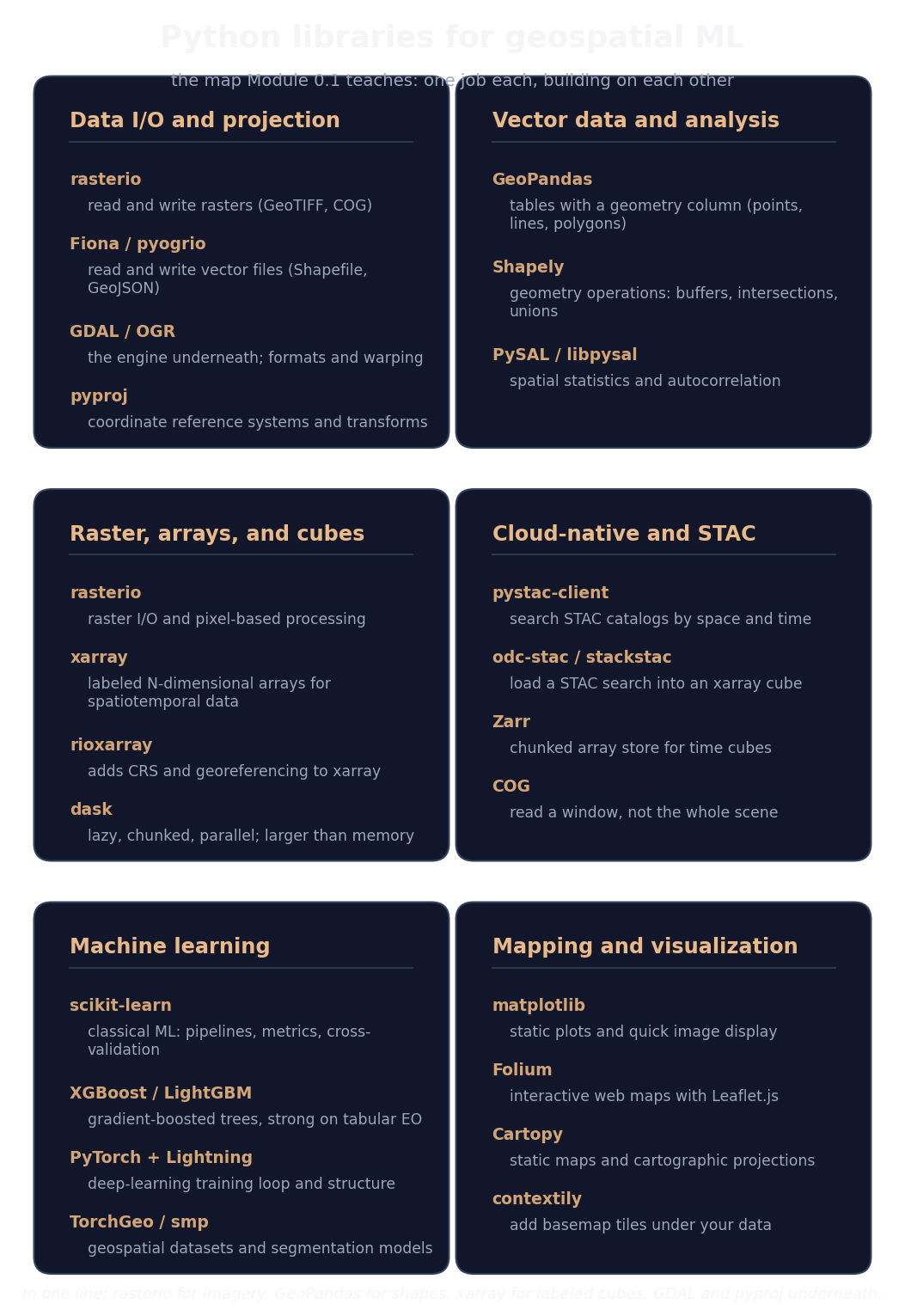
This is the mental map that prevents months of confusion. The geospatial stack is a small number of libraries that each do one job and build on each other.

• GDAL is the engine underneath almost everything. It reads and writes hundreds of raster and vector formats and does the low-level work of reprojection. You rarely call it directly, but when an install breaks, it is usually GDAL, which is why the conda route exists.
• rasterio is the friendly Python interface to GDAL for raster data (imagery). You use it to open a GeoTIFF, read pixels into a numpy array, and read the georeferencing (where each pixel sits on Earth).
• GeoPandas handles vector data (points, lines, polygons) as a table with a geometry column. It sits on top of shapely (geometry operations) and pyogrio/fiona (reading vector files). You use it for fire perimeters, administrative boundaries, and sample points.
• pyproj handles coordinate reference systems and transformations between them (more on CRS in Module 0.3).
• xarray is numpy with labeled axes and metadata. Instead of remembering that axis 0 is time and axis 2 is longitude, you name them. This becomes essential in Module 1 when you work with image time-series cubes, so we introduce the name now and go deep later.

A one-sentence summary to memorize: rasterio for imagery, GeoPandas for shapes, xarray for labeled cubes, GDAL and pyproj doing the heavy lifting underneath.

Guided lab (about 5 hours): build the eo-portfolio repository

You will create the repository the whole course commits into, wire up tests and CI, and prove the toolkit works by opening a raster and a vector and plotting them.

Step 1: Create the environment

Create a project folder and an environment. Using conda/mamba (most reliable for GDAL):

mamba create -n eo python=3.12 rasterio geopandas xarray rioxarray matplotlib numpy pandas pytest ruff pre-commit jupyterlab
mamba activate eo

Or with uv (verify current usage at install time):

uv init eo-portfolio && cd eo-portfolio
uv add rasterio geopandas xarray rioxarray matplotlib numpy pandas pytest ruff pre-commit jupyterlab

Export the environment to a file and commit it, so the setup is reproducible:

mamba env export --no-builds > environment.yml    # or rely on uv.lock with uv

Step 2: Initialize git and the repo layout

git init

Create this structure. The src/ layout is what professional Python packages use, and reviewers notice it:

eo-portfolio/
├── environment.yml            # or pyproject.toml + uv.lock
├── README.md
├── .gitignore                 # ignore data/, .ipynb_checkpoints/, __pycache__/
├── .pre-commit-config.yaml
├── src/eo_portfolio/
│   ├── __init__.py
│   └── io.py                  # small, tested helpers
├── tests/
│   └── test_io.py
├── notebooks/
│   └── 00_toolkit_check.ipynb
└── .github/workflows/ci.yml

Step 3: Write a small, tested helper

Put a genuinely useful function in src/eo_portfolio/io.py. It opens a raster and returns its basic metadata, the kind of check you run constantly:

"""Small IO helpers for the eo-portfolio course."""
from __future__ import annotations
import rasterio


def raster_summary(path: str) -> dict:
    """Open a raster and return its core spatial metadata.

    Returns width, height, band count, dtype, CRS as an EPSG string (or None),
    and the bounding box in the raster's own CRS.
    """
    with rasterio.open(path) as src:
        return {
            "width": src.width,
            "height": src.height,
            "bands": src.count,
            "dtype": src.dtypes[0],
            "crs": src.crs.to_string() if src.crs else None,
            "bounds": tuple(src.bounds),
        }

Step 4: Test it

In tests/test_io.py, write a tiny GeoTIFF into pytest's tmp_path so the test needs no external download, does not depend on any library's internal sample files, and runs anywhere in CI:

import numpy as np
import rasterio
from rasterio.transform import from_origin
from eo_portfolio.io import raster_summary


def test_raster_summary_reads_metadata(tmp_path):
    # Create a small 3-band GeoTIFF so the test is fully self-contained.
    path = tmp_path / "demo.tif"
    data = np.random.randint(0, 255, (3, 8, 8), dtype="uint8")
    transform = from_origin(0, 8, 1, 1)  # west, north, pixel x-size, pixel y-size
    with rasterio.open(
        path, "w", driver="GTiff", height=8, width=8, count=3,
        dtype="uint8", crs="EPSG:4326", transform=transform,
    ) as dst:
        dst.write(data)
    info = raster_summary(str(path))
    assert info["bands"] == 3
    assert info["width"] == 8 and info["height"] == 8
    assert info["crs"] is not None
    assert len(info["bounds"]) == 4

Run it locally until green:

pytest -q

Step 5: The toolkit-check notebook

In notebooks/00_toolkit_check.ipynb, prove the whole stack works end to end:

import numpy as np
import rasterio
from rasterio.plot import show
from rasterio.transform import from_origin
import geopandas as gpd
from geodatasets import get_path
from eo_portfolio.io import raster_summary

# Raster: make a tiny demo GeoTIFF, summarize, plot (no download needed)
demo = "demo.tif"
with rasterio.open(
    demo, "w", driver="GTiff", height=32, width=32, count=3, dtype="uint8",
    crs="EPSG:4326", transform=from_origin(0, 32, 1, 1),
) as dst:
    dst.write(np.random.randint(0, 255, (3, 32, 32), dtype="uint8"))
print(raster_summary(demo))
with rasterio.open(demo) as src:
    show(src)

# Vector: load a real-world dataset via geodatasets, inspect, plot
nybb = gpd.read_file(get_path("nybb"))   # New York City boroughs
print(nybb.crs, nybb.shape)
nybb.plot(column="BoroName", legend=True, figsize=(7, 6))

Note the history here, because it is exactly the currency habit this course teaches: geopandas.datasets (the old naturalearth_lowres shortcut) was removed in GeoPandas 1.0, so tutorials that still call it now break. The maintained replacement is the small geodatasets package (pip install geodatasets, then get_path("nybb") or another of its keys). If you would rather avoid the dependency, read any small boundary file directly, for example gpd.read_file("https://naciscdn.org/naturalearth/110m/cultural/ne_110m_admin_0_countries.zip"). The point is the same: open a vector, print its CRS and shape, and plot it, and verify what your installed versions actually provide rather than trusting a tutorial.

Step 6: Continuous integration

Add .github/workflows/ci.yml so every push runs your tests automatically. A minimal version:

name: ci
on: [push, pull_request]
jobs:
  test:
    runs-on: ubuntu-latest
    steps:
      - uses: actions/checkout@v4
      - uses: conda-incubator/setup-miniconda@v3
        with:
          environment-file: environment.yml
          activate-environment: eo
      - shell: bash -l {0}
        run: |
          pip install -e .
          ruff check src tests
          pytest -q

Add a .pre-commit-config.yaml that runs ruff before each commit so your code stays clean. Then:

pre-commit install
git add -A && git commit -m "Module 0.1: eo-portfolio scaffold with tested IO helper and CI"
git push

Confirm the green check mark appears on GitHub. That badge is the first thing a reviewer sees.

Checkpoint

Self-check (answers below).

1. Why do we create a separate environment per project instead of installing everything globally?
2. What is the difference between a numpy array and a pandas DataFrame, and which would you use for a Sentinel-2 image versus a table of GEDI footprints?
3. You need to open a GeoTIFF and read its pixels into an array. Which library, and why not GDAL directly?
4. What is the one-sentence summary of the geospatial library map?

Interview-style questions (practice out loud).

• A teammate says "my notebook works but yours crashes on the same code." What are the first two things you check?
• Why does a repository with tests and CI signal seniority more than a folder of notebooks, even if the science is identical?

Answers. (1) Isolation and reproducibility: different projects need different, often conflicting, package versions, and a committed environment file lets anyone recreate the exact setup. (2) numpy is an unlabeled n-dimensional array, ideal for the pixel grid of a Sentinel-2 image; pandas is a labeled table, ideal for GEDI footprints where each row is a point with named attributes. (3) rasterio, because it is the Pythonic interface to GDAL: fewer lines, safer file handling, and direct numpy output, while GDAL's own API is low level and verbose. (4) rasterio for imagery, GeoPandas for shapes, xarray for labeled cubes, GDAL and pyproj underneath.

Deliverable

A public eo-portfolio repository containing: a committed environment file, a src/ package with a tested raster_summary helper, a toolkit-check notebook that plots a raster and a vector, and a passing CI workflow (green badge). This is the spine every later module builds on.

What a hiring manager sees

At this stage the science is trivial, but the signal is not. A reviewer glancing at this repo sees an environment file (you understand reproducibility), a src/ layout with tests (you write software, not just scripts), and a green CI badge (your code runs somewhere other than your laptop). Many applicants with stronger models never show these basics. Leading with them frames everything that follows as the work of an engineer.

Currency note

Library names here (rasterio, GeoPandas, xarray, GDAL, pyproj, ruff, pre-commit) are stable and current as of the build date. Small API details drift, and a concrete example is already in this module: geopandas.datasets was removed in GeoPandas 1.0, so the naturalearth_lowres shortcut no longer exists and we use the geodatasets package instead (add it to your environment file). Verify the current recommended Python version and any pinned package versions at install time and record them in your environment file. This "verify, then pin" habit is the same one the SAR and foundation-model modules will demand, where mission and model status change fast.