Module 0.2: How Earth Observation Works
Phase: 0, Foundations
Level: Beginner
Estimated time: 6 to 8 hours
Prerequisites: Module 0.1 (your toolkit and eo-portfolio repo). No physics background required.
Portfolio thread: produces a sensor-and-mission cheat sheet and your first real scene pull, both committed to eo-portfolio. It gives you the mental model every later module assumes.
Why this module
You cannot reason about burn severity or radar backscatter until you know what a satellite actually measures. Most beginners jump straight to code and stay confused about why an optical image is empty under clouds, why one sensor sees a fire that another misses, or why "resolution" means four different things. This module builds the mental model of Earth observation so that from Module 1 onward the hard part is method, not confusion about the data. In interviews, the people who can explain sensor trade-offs in plain language read as engineers, not button-pushers.
Learning outcomes
After this module you can:
- Explain passive versus active remote sensing and give an example of each.
- Describe the regions of the electromagnetic spectrum used in EO and what each one reveals about the ground.
- Define the four resolutions (spatial, spectral, temporal, radiometric) and the trade-offs among them.
- Name the major open EO missions and say what each is good for.
- Explain data processing levels and what "analysis-ready" means.
- Register for the main data portals and pull your first scene over your study area.
Concept lessons (about 3.5 hours)
Lesson 1: How a satellite "sees"
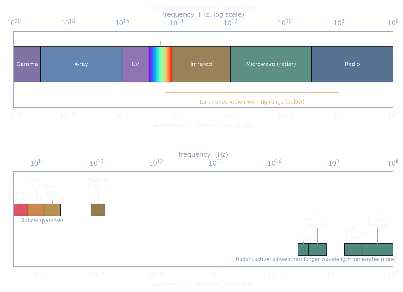
Remote sensing measures electromagnetic energy. The Sun floods the Earth with energy across a spectrum; surfaces reflect some of it and emit their own (as heat). A sensor in orbit records how much energy arrives in specific wavelength ranges called bands. Wavelength and frequency are two views of the same wave, linked by c = wavelength x frequency (c is the speed of light), so a shorter wavelength means a higher frequency and more energy. Earth observation uses only a small slice of the full spectrum, shown below.
Two families matter:
- Passive sensors record energy that already exists: sunlight reflected off the surface (optical) or heat emitted by the surface (thermal). They need the Sun (optical) and a clear sky, because clouds block these wavelengths.
- Active sensors send their own energy and measure what bounces back. Radar (Sentinel-1) sends microwaves; lidar (GEDI, ICESat-2) sends laser pulses. Because they supply their own signal and use long wavelengths, radar sensors see through clouds and work day or night. This is the single most important reason SAR exists in fire and forest monitoring.
The spectrum regions you will use, with their wavelength and frequency ranges and what each reveals:
- Visible (0.4 to 0.7 micrometres, about 430 to 750 THz): blue, green, and red, what the eye sees; true-color imagery.
- Near-infrared, NIR (about 0.7 to 1.3 micrometres): healthy vegetation reflects NIR strongly; the basis of NDVI and vegetation health.
- Shortwave infrared, SWIR (about 1.3 to 2.5 micrometres): sensitive to moisture and to char and ash after fire; the reason burn indices use SWIR.
- Thermal infrared (about 8 to 14 micrometres): surface temperature and, in the mid-infrared near 3.7 to 4 micrometres, active-fire heat.
- Microwave (radar), roughly 1 centimetre to 1 metre (about 0.3 to 30 GHz): surface roughness, structure, and moisture, and cloud-penetrating. The radar sub-bands, from shorter to longer wavelength, are X (about 3 cm, 8 to 12 GHz), C (3.8 to 7.5 cm, 4 to 8 GHz; Sentinel-1 is 5.6 cm at 5.405 GHz), L (15 to 30 cm, 1 to 2 GHz; NISAR is about 24 cm at 1.257 GHz), and P (30 to 100 cm, 0.3 to 1 GHz; ESA Biomass is about 70 cm at 435 MHz). Longer wavelength penetrates deeper, which is why C-band sees the canopy top while L-band and P-band reach branches, trunks, and soil.
One more reason these particular bands are used: the atmosphere is only transparent in certain "windows." The visible, parts of the infrared, and the microwave region pass through; much of the ultraviolet and many infrared wavelengths are absorbed. Clouds block the visible and much of the infrared but are nearly transparent to microwaves, which is the physical reason radar sees through cloud and works day or night.
A useful habit: whenever you pick an index or a sensor later, ask "which part of the spectrum am I relying on, and does it see the thing I care about?"
Lesson 2: The four resolutions and their trade-offs
"Resolution" means four different things, and they trade against each other.
- Spatial: ground size of one pixel (for example 10 m for Sentinel-2, 30 m for Landsat, 250 m to 1 km for MODIS/VIIRS). Smaller pixels show more detail.
- Spectral: how many and how narrow the bands are. More bands reveal more about material, at the cost of storage and complexity.
- Temporal (revisit): how often the sensor images the same place (days for Sentinel-2, sub-daily for MODIS/VIIRS). Frequent revisit matters for fast events like fire.
- Radiometric: how finely brightness is recorded (bit depth). Higher radiometric resolution distinguishes subtle differences.
The trade-off to internalize: you rarely get high spatial, high spectral, and high temporal resolution at once. A sensor with tiny pixels usually images a narrower strip less often; a sensor that sees the whole planet daily has coarse pixels. Choosing a data source is choosing which resolution matters most for the job. For a fast-moving fire you may accept coarse pixels for daily coverage; for mapping a burn scar's edges you want fine pixels and can wait for a clear pass.
Lesson 3: The major data sources
Learn these as a toolkit, not a list:
- Optical, medium resolution: Landsat (about 30 m, the longest continuous record, decades deep) and Sentinel-2 (about 10 m, frequent revisit). HLS (Harmonized Landsat and Sentinel) blends the two into one consistent optical series, which is why the burn-scar work later uses it.
- Optical, coarse and frequent: MODIS and VIIRS (hundreds of metres, at least daily). Coarse pixels, but their daily coverage makes them the backbone of active-fire detection.
- Radar: Sentinel-1 (C-band, all-weather, day and night). The go-to open SAR source for change and flood work.
- Lidar and altimetry: GEDI and ICESat-2 measure vegetation structure and elevation along tracks, not wall-to-wall; the basis of canopy-height and biomass work.
- Commercial, high resolution: providers such as Planet, Maxar, ICEYE, and Capella offer sub-metre optical or radar, usually paid. Useful when you need detail the open sensors cannot give.
The skill is matching source to question: daily fire detection points to VIIRS; a sharp burn-severity map points to HLS or Sentinel-2; cloud-proof change points to Sentinel-1; canopy height points to GEDI fused with imagery.
Lesson 4: Processing levels and analysis-ready data
Raw sensor data is not what you model on. Products come in levels:
- Level 0 and 1: raw or calibrated and geometrically corrected, but still top-of-atmosphere (affected by the atmosphere).
- Level 2: corrected to surface reflectance (optical) or a geophysical quantity, with quality and cloud-mask layers. This is usually where you start, because the atmosphere has been removed and pixels are comparable across dates.
- Higher levels and ARD: composites, mosaics, and "analysis-ready data" that are tiled, aligned, and cloud-screened so you can go straight to analysis.
Two rules of thumb: prefer surface-reflectance (Level 2) products for optical work, and always read and apply the quality or cloud mask that ships with the product. Skipping the mask is the most common source of silently wrong results.
Lesson 5: The application landscape, and where this course goes deep
Earth observation is applied across a huge range of fields, and it helps to see the whole map early, because the skills you build in this course transfer across almost all of it.
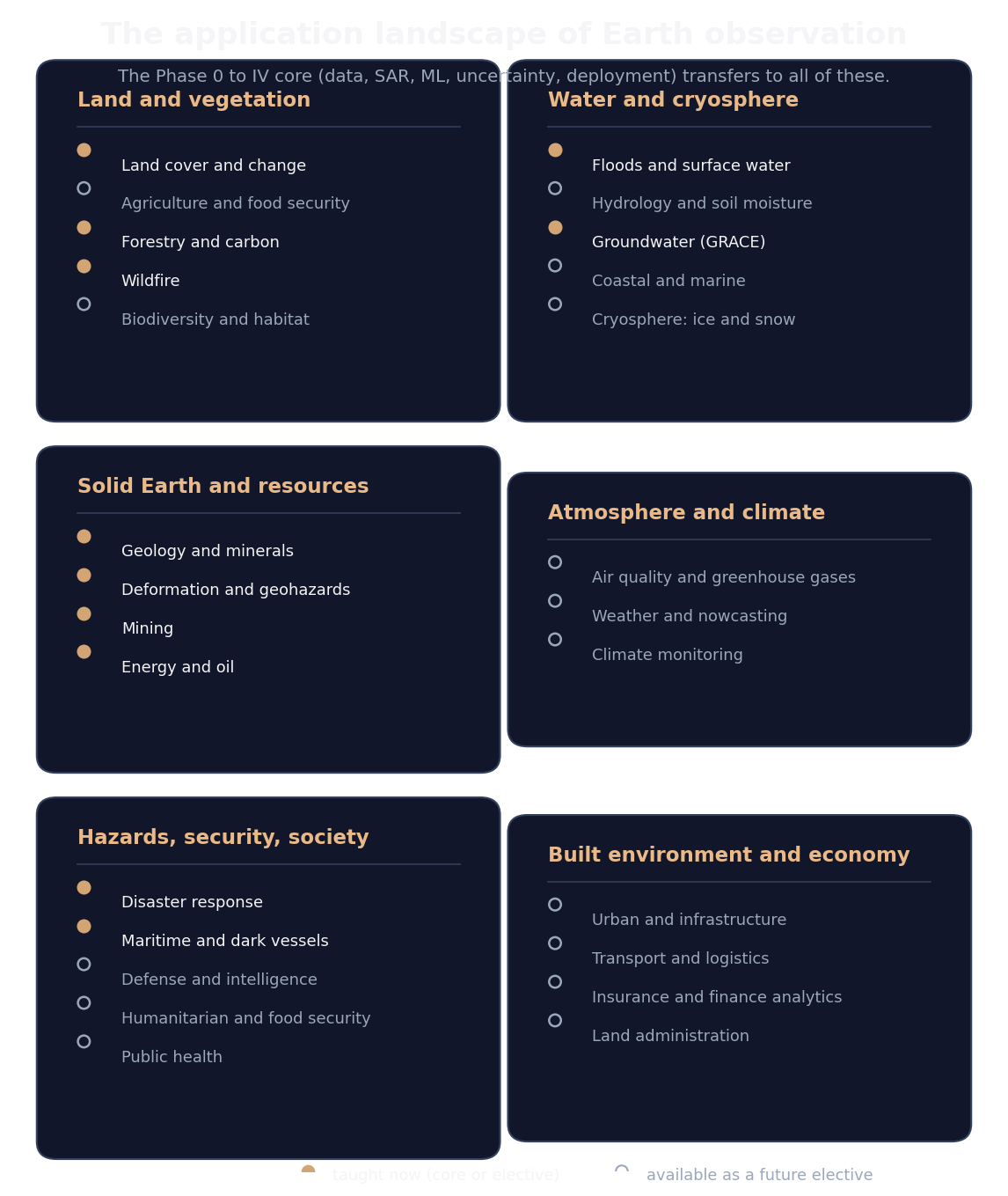
The important idea is that the core of this course is not "wildfire tricks." It is a transferable method spine: turn a cloud archive into an analysis-ready cube, engineer features or train a network, validate honestly with spatial cross-validation and uncertainty, and ship the result as a service. That spine is what agriculture, water, urban, coastal, air-quality, and disaster teams all use; only the data sources and the labels change.
This course goes deep on wildfire, forestry and carbon, SAR, and floods and hazards, because depth in a real niche is what gets you hired, and it adds optional electives (starting with geology and geophysics) so you can specialize toward the fields you want. When you finish the core, adapting to a new application is a matter of swapping the dataset and the target, not learning a new craft.
Guided lab (about 3 hours): accounts, a cheat sheet, and your first scene


Step 1: Register for the main data portals
Create free accounts (you will use these throughout the course):
- NASA Earthdata (register once; gives Landsat, MODIS/VIIRS, GEDI, HLS via Earthdata Login)
- Copernicus Data Space Ecosystem (register for Sentinel-1 and Sentinel-2)
- USGS EarthExplorer (register for the Landsat archive; browse at earthexplorer.usgs.gov)
- Microsoft Planetary Computer (open STAC catalog and cloud access; no account needed to read the public STAC)
Store any credentials with your password manager, never in the repo.
Step 2: Build a sensor cheat sheet
In eo-portfolio, add docs/sensors.md with a table you will actually reuse:
| Mission | Type | Key bands | Spatial | Revisit | Best for |
|---|---|---|---|---|---|
| Sentinel-2 | passive optical | visible, NIR, SWIR | ~10 m | frequent | burn severity, vegetation |
| Landsat | passive optical | visible, NIR, SWIR, thermal | ~30 m | ~16 days | long-term change |
| VIIRS | passive optical/thermal | thermal | ~375 m | sub-daily | active fire |
| Sentinel-1 | active radar (C-band) | VV, VH | ~10 to 20 m | frequent | all-weather change, flood |
| GEDI | active lidar | n/a | footprint | sparse tracks | canopy height, biomass |
Fill it in from the lesson and the mission docs, and add a one-line "when I would reach for this" note per row. This becomes a reference you use in every later module.
Step 3: Pull your first scene
Using your Module 0.1 toolkit, search a STAC catalog for a Sentinel-2 scene over your study-area fire AOI and describe it. This is a read-and-inspect exercise, not processing yet:
import pystac_client, planetary_computer

catalog = pystac_client.Client.open(
    "https://planetarycomputer.microsoft.com/api/stac/v1",
    modifier=planetary_computer.sign_inplace,
)
# a small bbox over your fire AOI (lon/lat): west, south, east, north
bbox = [-118.6, 34.0, -118.3, 34.2]
search = catalog.search(
    collections=["sentinel-2-l2a"],
    bbox=bbox,
    datetime="2025-01-01/2025-03-31",
    query={"eo:cloud_cover": {"lt": 20}},
)
items = list(search.items())
print("scenes found:", len(items))
best = min(items, key=lambda it: it.properties["eo:cloud_cover"])
print("id:", best.id)
print("date:", best.properties["datetime"])
print("cloud cover:", best.properties["eo:cloud_cover"])
print("bands:", sorted(best.assets.keys())[:12])
If Planetary Computer is unavailable to you, run the same search against the Copernicus Data Space STAC API. The point is to prove you can find the right scene and read its metadata (date, cloud cover, available bands). Save this as notebooks/01_first_scene.ipynb.
Step 4: Commit
git add docs/sensors.md notebooks/01_first_scene.ipynb
git commit -m "Module 0.2: sensor cheat sheet and first Sentinel-2 scene lookup"
git push
Checkpoint
Self-check (answers below).
- Why can Sentinel-1 image a flood at night through thick cloud when Sentinel-2 cannot?
- Your task is to detect new fires within hours across a whole country. Which resolution do you prioritize, and which sensor family fits?
- Why do burn indices rely on the SWIR band?
- You downloaded a Level 1 top-of-atmosphere product and your multi-date comparison looks noisy. What did you likely skip?
Interview-style questions (practice out loud).
- Explain passive versus active remote sensing to a product manager in three sentences.
- A stakeholder asks for "the highest resolution data, updated daily, with lots of bands." What is wrong with the request, and how do you reframe it?
Answers. (1) Sentinel-1 is active radar using long microwaves that penetrate cloud and need no sunlight, while Sentinel-2 is passive optical that depends on reflected sunlight and is blocked by cloud.
(2) Prioritize temporal resolution (frequent revisit); the coarse but sub-daily VIIRS/MODIS family fits, accepting large pixels for speed.
(3) SWIR is sensitive to moisture and to char and ash, so it drops sharply where vegetation burned, making the pre-minus-post difference a strong burn signal.
(4) You likely skipped surface-reflectance correction and the cloud/quality mask; use a Level 2 product and apply its mask so dates are comparable.
Deliverable
A committed docs/sensors.md cheat sheet and a notebooks/01_first_scene.ipynb that finds and describes one low-cloud Sentinel-2 scene over your study-area AOI (date, cloud cover, bands). This is the reference and the first data touch the rest of the course builds on.
What a hiring manager sees
Anyone can run a model on a dataset someone handed them. Being able to reason about sensor and resolution trade-offs, and to justify why you chose a data source for a given question, is what distinguishes an EO engineer from a general ML practitioner. A tidy sensor cheat sheet and a clean scene-lookup notebook show that judgment early.
Currency note
The concepts here (passive versus active, the spectrum, the four resolutions, processing levels) are stable. The wavelength and frequency ranges use the IEEE radar band designations (X 8 to 12 GHz, C 4 to 8 GHz, L 1 to 2 GHz, P 0.3 to 1 GHz) and the published centre frequencies of Sentinel-1 (5.405 GHz), NISAR L-band (1.257 GHz), and ESA Biomass (435 MHz), verified August 2026; the electromagnetic-spectrum figure is an original diagram (no third-party image). Mission specifics such as exact revisit, band lists, and which sensors are currently operational do drift as satellites launch and retire, so verify a mission's current status and characteristics from its official documentation at study time, and confirm the STAC endpoints and collection names before running the lab.