Module 0.3: Geospatial Data 101 (Raster, Vector, and CRS)

Phase: 0, Foundations
Level: Beginner
Estimated time: 7 to 9 hours
Prerequisites: Modules 0.1 (toolkit) and 0.2 (how EO works).
Portfolio thread: adds a tested geo.py helper module (reproject, clip, rasterize, UTM picker) and a first map figure to eo-portfolio. These utilities are used in almost every later module.

Why this module

Almost every EO bug eventually traces to one of three things: a coordinate system mismatch, a resolution or grid misalignment, or confusing raster with vector. Get these fundamentals right and you avoid the errors that quietly corrupt results, like computing area in degrees or resampling a category map with the wrong method. This is also the exact material a live-coding interview probes, because it separates people who can move geospatial data around correctly from people who produce maps that look fine and are silently wrong.

Learning outcomes

After this module you can:

Explain raster versus vector and choose the right one for a task.
Read and reason about a coordinate reference system: geographic versus projected, EPSG codes, UTM, and when to reproject.
Describe raster anatomy: the affine transform, bounds, pixel size, nodata, dtype, and bands.
Perform the core operations: reproject, clip to an area of interest, resample with the correct method, rasterize a vector, and vectorize a raster.
Work with vector data: geometries, attributes, spatial joins, and area computed correctly.
Ship a tested geo.py module and a map figure.

Concept lessons (about 4 hours)

Lesson 1: Raster versus vector

Two data models cover almost everything in EO.

Raster: a grid of equally sized cells, each holding a value. Imagery, elevation models, temperature fields, and classification maps are rasters. Rasters are ideal for continuous surfaces and for anything a sensor measures pixel by pixel.
Vector: discrete shapes, points, lines, and polygons, each with attributes. Fire perimeters, administrative boundaries, roads, and sample locations are vectors. Vectors are ideal for objects with clear edges and for tabular attributes attached to places.

You constantly convert between them: rasterize a perimeter polygon into a mask to apply to imagery, or vectorize a burned-area raster into polygons to report area. Knowing which model fits, and converting deliberately, is half the job.

Lesson 2: Coordinate reference systems

A CRS tells you what the coordinates mean. This is the single most common source of confusion, so slow down here.

Geographic CRS: coordinates are longitude and latitude in degrees, on a model of the globe. The common one is EPSG:4326 (WGS84). Degrees are not a constant distance on the ground, so you cannot measure area or distance reliably in a geographic CRS.
Projected CRS: the curved Earth is flattened onto a plane so coordinates are in metres. UTM divides the world into 6-degree zones, each an accurate local metric system; EPSG:3857 (Web Mercator) is the projection web maps use, good for display but distorted for area.
Datum: the reference model of the Earth's shape (WGS84 is standard). Mixing datums causes small but real misalignment.

The rules that prevent most bugs: to measure area or distance, reproject to an appropriate projected CRS (usually the local UTM zone) first; to overlay two layers, make sure they share a CRS; and remember that reprojecting a raster resamples it, which slightly changes pixel values, so reproject as few times as possible and keep a canonical grid. The classic bug, "my layers do not line up," is almost always two different CRSs or a datum mismatch.

Picking the UTM zone from a longitude is a formula you will reuse:

def pick_utm_epsg(lon: float, lat: float) -> int:
    """EPSG code of the UTM zone containing (lon, lat). 326xx north, 327xx south."""
    zone = int((lon + 180) // 6) + 1
    return (32600 if lat >= 0 else 32700) + zone

Lesson 3: Raster anatomy and operations

A raster is an array plus georeferencing. The georeferencing is an affine transform: six numbers that map a pixel's row and column to a coordinate on the ground. From it you get the top-left origin, the pixel size, and the bounds. The other essentials are the CRS, the data type (dtype), the band count, and the nodata value that marks empty pixels so they are excluded from math.

The core operations:

Read a window: load just a sub-region, so you never download or hold a whole scene to work on a small area. This is why cloud-optimized GeoTIFFs matter.
Reproject (warp): change the CRS, which resamples onto a new grid.
Clip or mask: cut a raster to a polygon (a fire AOI, for example).
Resample: change resolution or align grids. Method matters: use nearest-neighbour for categorical rasters (class labels, because averaging classes is meaningless) and bilinear or cubic for continuous rasters (reflectance, elevation). Using nearest on continuous data throws away accuracy; using bilinear on categories invents nonexistent classes.
Rasterize and polygonize: convert a vector to a raster mask, or a raster to vector polygons.

Lesson 4: Vector operations

A GeoDataFrame is a table with a geometry column and a CRS. The operations you need early:

Attributes and filtering: select rows by attribute, just like a normal table.
Spatial predicates: test relationships such as intersects, within, and contains.
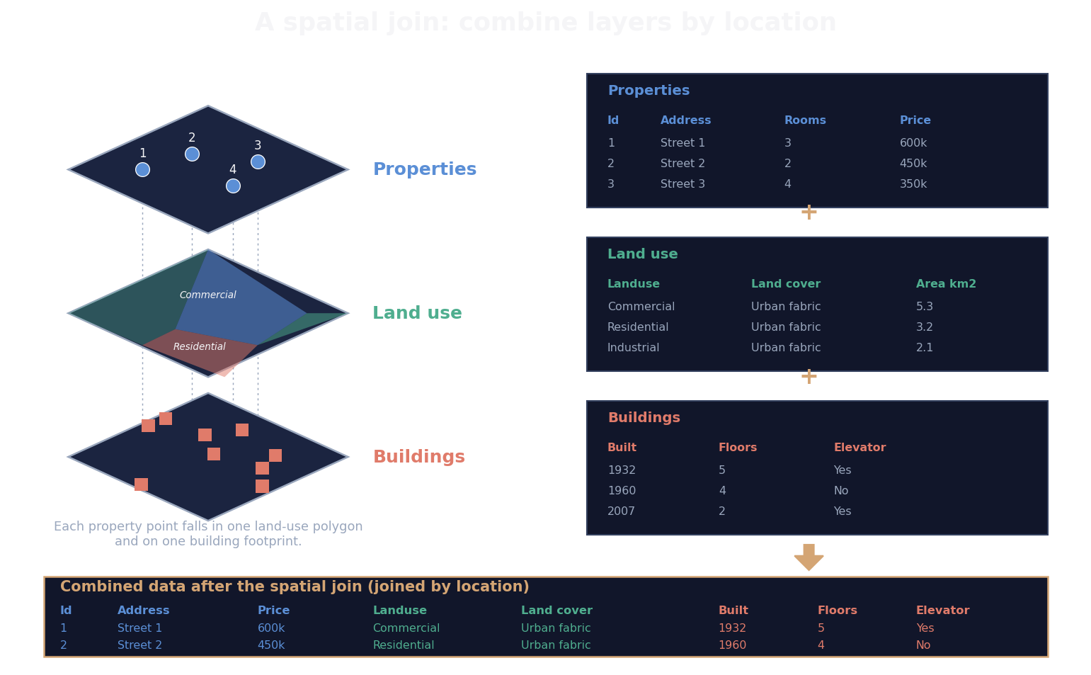
Spatial join: attach attributes from one layer to features of another based on location (for example, label sample points by which AOI they fall in).
Dissolve and buffer: merge features by a key, or grow a geometry by a distance (buffers need a projected CRS to be in metres).
Area and length: compute only in a projected CRS, never in degrees.

The spatial join is the one to picture clearly, because you will use it constantly to attach context to points (for example, tagging each sample or property with the land-use polygon and building it falls on):

Three layers (property points, land-use polygons, building footprints) with their attribute tables combined into one table by location — A spatial join combines layers by location: each property point takes the attributes of the land-use polygon and building footprint it falls within, producing one merged table. The match is by geometry (which point is inside which polygon), not by row order.

Guided lab (about 4 hours): a tested `geo.py` and a map

Build src/eo_portfolio/geo.py with small, tested helpers you will reuse all course long.

Step 1: The helpers

"""Geospatial helpers for the eo-portfolio course."""
from __future__ import annotations
import geopandas as gpd
import rasterio
from rasterio.warp import calculate_default_transform, reproject, Resampling
from rasterio.features import rasterize


def pick_utm_epsg(lon: float, lat: float) -> int:
    """EPSG code of the UTM zone containing (lon, lat)."""
    zone = int((lon + 180) // 6) + 1
    return (32600 if lat >= 0 else 32700) + zone


def area_ha_utm(gdf: gpd.GeoDataFrame) -> float:
    """Total area of a GeoDataFrame in hectares, computed in the correct UTM zone."""
    c = gdf.to_crs(4326).union_all().centroid
    utm = pick_utm_epsg(c.x, c.y)
    return gdf.to_crs(utm).area.sum() / 10_000.0


def rasterize_like(gdf: gpd.GeoDataFrame, transform, out_shape, fill=0, value=1):
    """Burn vector geometries onto a grid defined by transform + out_shape."""
    shapes = ((geom, value) for geom in gdf.geometry)
    return rasterize(shapes, out_shape=out_shape, transform=transform,
                     fill=fill, dtype="uint8")

(Reprojecting a raster with rasterio.warp.reproject, or more simply rioxarray's .rio.reproject, is worth adding too; keep whichever you use covered by a test.)

Step 2: Tests that need no downloads

import numpy as np
from shapely.geometry import box
import geopandas as gpd
from rasterio.transform import from_bounds
from eo_portfolio.geo import pick_utm_epsg, area_ha_utm, rasterize_like


def test_utm_zone_picks_correctly():
    assert pick_utm_epsg(-118.4, 34.1) == 32611   # Los Angeles, UTM 11N
    assert pick_utm_epsg(7.5, 5.0) == 32632        # Niger Delta, UTM 32N
    assert pick_utm_epsg(151.2, -33.9) == 32756    # Sydney, UTM 56S


def test_area_ha_is_reasonable():
    # a ~0.01 x 0.01 degree box near the equator is roughly 100+ ha
    gdf = gpd.GeoDataFrame(geometry=[box(7.50, 5.00, 7.51, 5.01)], crs=4326)
    a = area_ha_utm(gdf)
    assert 90 < a < 140


def test_rasterize_covers_center():
    gdf = gpd.GeoDataFrame(geometry=[box(0.25, 0.25, 0.75, 0.75)], crs=4326)
    transform = from_bounds(0, 0, 1, 1, 10, 10)
    mask = rasterize_like(gdf, transform, (10, 10))
    assert mask.sum() > 0 and mask[5, 5] == 1

Run until green: pytest -q.

Step 3: A real overlay and a map

In notebooks/02_geo_basics.ipynb: load your study-area fire perimeter (or any polygon) with GeoPandas, print its CRS, reproject to the correct UTM zone, and compute its area in hectares with area_ha_utm. Then open the Sentinel-2 scene from Module 0.2, clip it to the AOI, and plot the clipped true-color image with the perimeter drawn on top. Save the figure to docs/aoi_map.png.

Step 4: Commit

git add src/eo_portfolio/geo.py tests/test_geo.py notebooks/02_geo_basics.ipynb docs/aoi_map.png
git commit -m "Module 0.3: tested geo helpers (UTM, area, rasterize) + AOI map"
git push

Checkpoint

Self-check (answers below).

Why must you reproject to a projected CRS before computing a polygon's area?
You are resampling a land-cover class map to a finer grid. Which resampling method, and why not bilinear?
What does the affine transform of a raster actually do?
Two layers that should overlap are drawn far apart on your map. What is the first thing you check?

Interview-style questions (practice out loud).

Given a cloud-optimized GeoTIFF on cloud storage, how do you read one 512 by 512 window without downloading the whole file, and why is that possible?
Walk through computing the area of a mining or burn polygon correctly, including the CRS choice.
When would you rasterize a vector, and when would you vectorize a raster?

Answers. (1) A geographic CRS measures in degrees, which represent different ground distances at different latitudes, so area in degrees is meaningless; a projected CRS (usually the local UTM zone) measures in metres.
(2) Nearest-neighbour, because class labels are categorical and averaging them (as bilinear does) invents classes that do not exist.
(3) It maps pixel row and column indices to real-world coordinates (origin, pixel size, and orientation), so the array knows where each cell sits on Earth.
(4) Whether the two layers share the same CRS (and datum); a CRS mismatch is the usual cause of layers not lining up.

Deliverable

A tested src/eo_portfolio/geo.py (UTM picker, correct area, rasterize) with a passing tests/test_geo.py, plus notebooks/02_geo_basics.ipynb and a saved docs/aoi_map.png showing your AOI over a clipped Sentinel-2 image. Foundations complete: you now have the toolkit, the mental model, and the geospatial fundamentals to start Phase I.

What a hiring manager sees

CRS fluency and correct resampling and area handling are exactly what live-coding rounds test, because they are where careless work produces confidently wrong maps. A small, tested geo.py with a correct UTM area function and a clean AOI map signals that you will not ship silently broken geospatial results, which is worth more to a hiring manager than another model.

Currency note

These fundamentals are stable. Library function signatures evolve slightly (for example rasterio.warp.reproject, rioxarray's .rio.reproject, and the GeoPandas union_all versus older unary_union), so confirm the current API of any function you call against its documentation at study time, and pin your versions in the environment file from Module 0.1.