Module 9.6: Resources, Minerals, and Energy from Space

Phase: III elective (Geology and Geophysics from Space)
Level: Advanced · Optional
Estimated time: ~18 to 20 hours (about 6 h concepts, 11 h across two labs, 1 to 2 h write-up). The hyperspectral MTMF and the CNN lithology steps are marked stretch; the core path is closer to 15 hours.
Prerequisites: Modules 4 (classical ML and spatial cross-validation), 5 (uncertainty), and 9.5 (structure and deformation). Phase 0.
Portfolio thread: a lithology and alteration map over a greenstone or basement terrain, and a mineral-prospectivity or landslide-susceptibility map with uncertainty and an area-of-applicability check. Second half of the optional Geology and Geophysics elective.

Why this module

The mineral and energy transition runs on finding things in the ground, and the discovery rate has been falling for decades, which is exactly why AI-first explorers have attracted serious money. KoBold Metals (valued around 4.4 billion dollars in 2026, with a copper discovery in Zambia and platforms called TerraShed and Machine Prospector), Earth AI, and Fleet Space frame exploration as a data-fusion problem: combine imagery, terrain, and geophysics to rank where to drill. Mining majors and juniors, geological surveys, consultancies, and energy and geothermal operators hire people who can do this responsibly, which means honest uncertainty and a clear statement of where a model should not be trusted. This module surveys the resource applications and goes deep on two workhorse skills: spectral mineral mapping and prospectivity or susceptibility modelling with an area-of-applicability check.

Learning outcomes

After this module you can:

1. Map minerals and alteration with multispectral band ratios and indices (iron oxide, clay, carbonate) and know their limits, including the fact that ASTER SWIR has not worked since 2008.
2. Use hyperspectral data (EMIT, EnMAP, PRISMA) with the Spectral Angle Mapper and the USGS spectral library, and know when the products are and are not suitable for exploration.
3. Classify lithology with random forests, design a defensible geological sample, and use field maps and drillholes as labels.
4. Build a mineral-prospectivity or landslide-susceptibility map that fuses imagery, DEM derivatives, and open geophysics, with weights of evidence and random forests, spatial cross-validation, and an area-of-applicability check.
5. Monitor mining and energy from space: artisanal and illegal mining, open-pit and tailings deformation, methane and thermal anomalies, and reservoir and storage deformation, and connect these to ESG and MRV reporting.
6. Ship tested helpers and two maps with honest uncertainty, and speak to the current industry landscape.

Concept lessons (about 6 hours)

Lesson 1: Multispectral mineral mapping and its limits

Broadband sensors cannot identify minerals, but they detect diagnostic absorption features through band ratios:

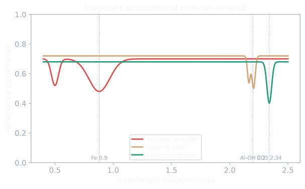
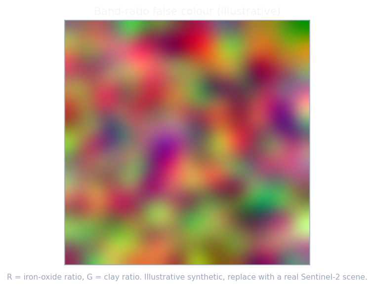
• Iron oxides (hematite, goethite) absorb in the blue and reflect in the red, so a red-over-blue ratio (Sentinel-2 B4/B2, Landsat equivalents) highlights them.
• Clays, micas, and carbonates have absorptions in the shortwave infrared near 2.2 and 2.3 microns, so SWIR ratios (Sentinel-2 B11 and B12) give a coarse alteration proxy.
• ASTER historically gave finer SWIR mineral ratios, but its SWIR detectors failed in April 2008 and are permanently off, so any ASTER SWIR mineral work must use the pre-2008 archive; ASTER TIR (for silica and carbonate) and VNIR still work. This is a classic trap: code that pulls current ASTER SWIR returns saturated, striped garbage.

Regolith and laterite cover, common across West Africa, both helps (iron and clay signatures are strong) and hinders (thick cover hides bedrock), so interpret indices as surface mineralogy, not bedrock geology, and calibrate to field observations.

Lesson 2: Hyperspectral and the Spectral Angle Mapper

Imaging spectrometers measure hundreds of contiguous bands, enough to identify minerals by their absorption shapes:

• Missions: EMIT on the ISS (open, VSWIR, targeted coverage, operating through at least 2026), EnMAP (German, nominal end of life around September 2026) and PRISMA (Italian), both tasked, and a growing set of upcoming missions. EMIT is the most accessible open source, but check tile coverage over your area of interest, since it does not image everywhere.
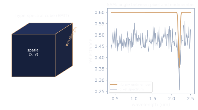
• Methods: the Spectral Angle Mapper compares a pixel spectrum to a library reference by the angle between them, which is invariant to brightness (illumination and slope), so it is robust for mineral matching. Matched Filtering and MTMF, endmember extraction, and, increasingly, deep learning on the full cube go further. The reference spectra come from the USGS Spectral Library Version 7.

• A crucial honesty point: EMIT ships an L2B mineralogy product (the EMIT-10 minerals: calcite, chlorite, dolomite, goethite, gypsum, hematite, illite plus muscovite, kaolinite, montmorillonite, vermiculite), but it was built to constrain dust radiative forcing, and NASA explicitly cautions that the maps need further validation before use in resource exploration. Use it as a strong starting point that you validate, not as a finished exploration product.

Lesson 3: Lithological classification and geological sampling

Predicting rock type from imagery is a supervised classification with a geological twist:

• Labels come from published geological maps, field stations, and drillholes, all of which are sparse, biased to accessible ground, and sometimes wrong at the boundary. Treat labels as imperfect and weight your validation toward independent field checks.
• Features are the Module 4 stack (optical composites and indices, Sentinel-1 backscatter and ratio, DEM derivatives) plus the spectral indices above.
• Models: random forests are the strong, interpretable baseline; CNNs on image patches help where texture and context matter (a stretch step). The Module 4 discipline is non-negotiable here, because geology is strongly spatially autocorrelated and a random split will flatter you badly.

Lesson 4: Prospectivity, fusing imagery with geophysics

Mineral prospectivity mapping ranks where a deposit type is likely, by fusing many evidence layers:

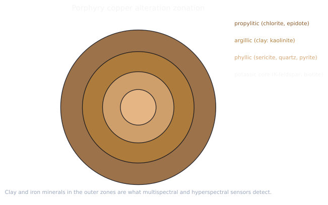
• Deposit models tell you what to look for: porphyry copper (large alteration halos), epithermal gold (silica and clay alteration), orogenic gold (structural control along shears), and lithium (pegmatites or brines). Each implies different evidence.

• Geophysics is the other half of the data. Airborne magnetics (magnetic minerals and structure), radiometrics (potassium, thorium, uranium for alteration and rock type), gravity (density, intrusions), and electromagnetics (conductors) are the exploration workhorses. The key constraint is what is openly reproducible where you work. For Nigeria, high-resolution airborne coverage exists (the Nigerian Geological Survey Agency flew nationwide magnetic and radiometric surveys at 500 metre line spacing), but it is delivered through a paid, order-based system, so a self-paced learner cannot build a lab on it. What you can use openly over Nigeria are the coarse global grids: EMAG2v3, the 2 arc-minute (about 3.7 km) Earth Magnetic Anomaly Grid from NOAA, and WGM2012, the global Bouguer and free-air gravity grids from the Bureau Gravimetrique International. These resolve regional structure, basins, and large intrusions, not deposit-scale detail, so a Nigeria prospectivity map from them is an honest first-pass regional ranking, not a drill target. Where you need high-resolution open airborne magnetics, radiometrics, and gravity for a true deposit-scale exercise, Geoscience Australia publishes national grids for free, which is why this module offers an Australian district as the optional high-resolution comparison. Open global radiometrics do not exist at useful quality, so radiometrics is an Australia-only optional layer; state that rather than fake it.
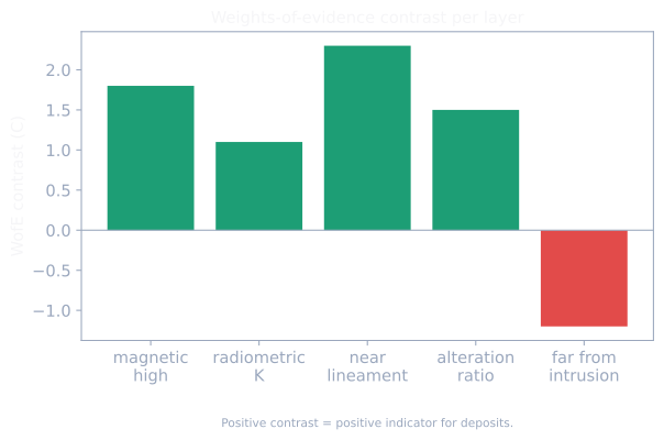
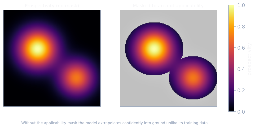
• Methods: weights of evidence is the classic transparent baseline (each layer gets a positive or negative weight and a contrast), random forests and gradient boosting are the modern workhorse, and CNNs and foundation-model embeddings are the frontier that KoBold and peers use. Whatever the model, a prospectivity map without an area-of-applicability mask is dangerous, because it will extrapolate confidently into ground unlike anything it was trained on.

Lesson 5: Mine and infrastructure monitoring

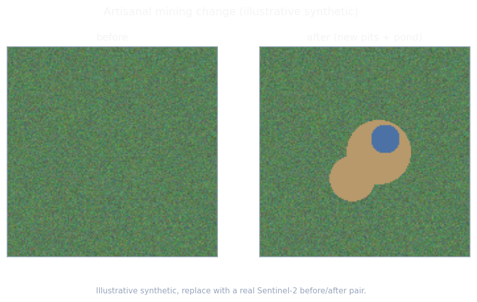
• Artisanal and illegal mining shows up as new bare-ground scars and turbid water in Sentinel-2 and as backscatter change in Sentinel-1, the same change-detection machinery as Module 6, and it connects directly to the illegal-mining monitoring that Lillie Earth Intelligence already does.

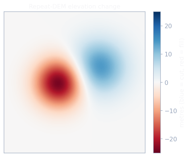
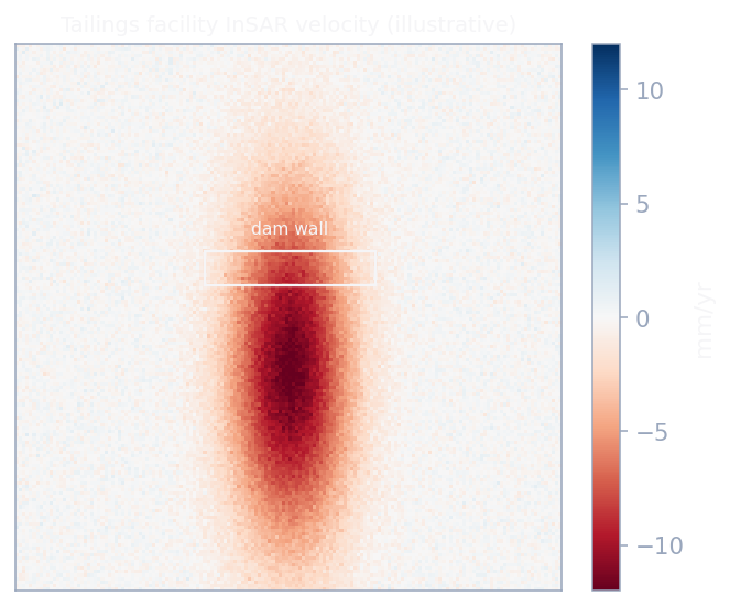
• Open-pit extent and volume change from repeat DEMs (differencing surfaces gives cut and fill volumes), and tailings storage facilities are monitored for deformation with InSAR (Module 9.5), a life-safety application after several catastrophic dam failures.

• Global context: the open Maus et al. global mining polygons (Version 2, from Sentinel-2, covering open cuts, tailings dams, waste rock, and ponds) give a worldwide footprint to sample from and validate against.

Lesson 6: Energy, water, and the ESG and MRV frame

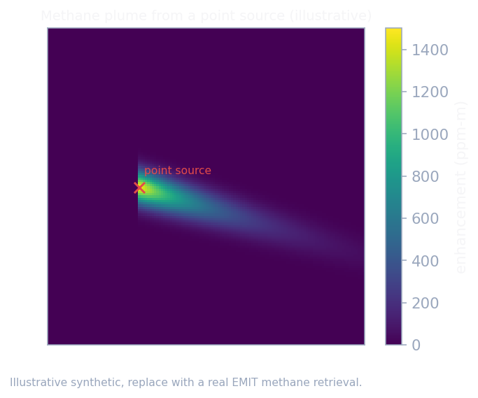
• Oil, gas, and geothermal: hydrocarbon seeps, methane plumes (TROPOMI at coarse scale for whole basins, EMIT for individual point sources), SO2, geothermal thermal anomalies (Landsat and ASTER TIR), and surface deformation over producing reservoirs and over CO2 storage sites (InSAR), which ties directly to the PipelineWatch-NG setting in the Niger Delta.
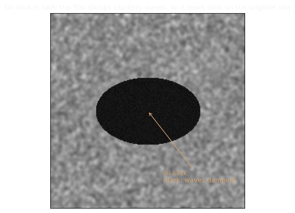
• Oil slicks and seeps with SAR: an oil film damps the sea's small capillary waves, so the surface becomes smooth relative to the radar wavelength and returns little energy. A slick therefore appears as a dark patch on the brighter wind-roughened sea in Sentinel-1, the inverse of the bright-ship case in Module 9. This is the workhorse method for spill response and natural-seep mapping, and it works through cloud and at night. Beware look-alikes (low-wind zones, algal films, rain cells), so use wind context and multi-temporal imagery. ICEYE markets oil-spill monitoring on exactly this signal.
• Crude oil storage from space: floating-roof storage tanks have a lid that rides on the oil, so its height changes with the fill level. Satellites read the shadow the tank wall and roof cast (SAR measures the roof geometry directly, optical reads the crescent shadow), and repeated imaging turns that into how full each tank is and, aggregated over a region, into crude-inventory estimates that move markets. This is the flagship SAR-for-oil analytic, and it is Ursa Space Systems' signature product (a global oil-storage index built from a virtual SAR constellation).
• Niger Delta specifics (PipelineWatch-NG): illegal bunkering and artisanal refining show as Sentinel-2 spill scars and blackened ground, as gas-flare thermal signatures (VIIRS Nightfire, Landsat and ASTER TIR), and as SAR slicks that cut through the region's persistent cloud. Fusing these is a concrete, high-value monitoring product and a direct extension of your existing work.

• Hydrogeology: basin-scale groundwater from GRACE and GRACE-FO (Module 9.5), plus wetland, spring, and karst mapping and soil moisture from optical and radar.
• Environmental geology and ESG: acid mine drainage and water-quality proxies, rehabilitation and revegetation monitoring, coastal erosion and cliff retreat, permafrost thaw, and dust and desertification. These are increasingly reported under ESG and measurement, reporting, and verification frameworks, so a remote-sensing geoscientist who can produce auditable change metrics is valuable beyond exploration.

A short foundation-model note: geospatial foundation models (Prithvi, Clay, TerraMind from Module 8) and physics-informed ML are entering geoscience, mostly as embedding features that feed the same prospectivity and classification pipelines rather than as end-to-end replacements. Name them correctly and treat them as one more evidence layer for now.

Guided lab (about 11 hours): two maps

A starter notebook notebooks/13_mineral_mapping.ipynb scaffolds the Sentinel-2 and EMIT pulls, and notebooks/14_prospectivity.ipynb scaffolds the geophysics fusion and cross-validation. You write the analysis.

Lab A: mineral and lithology mapping (about 5 hours)

Over a Nigerian schist belt (for example the Anka or Maru belt in the northwest) or a West African Birimian greenstone belt, and compared against an Australian or Nevada porphyry district:

1. Pull Sentinel-2 L2A and compute the iron-oxide (B4/B2) and clay or carbonate (B11/B12) ratios and a relative absorption band depth. Add the Copernicus GLO-30 DEM derivatives from Module 9.5.
2. If an EMIT tile covers your area, run a Spectral Angle Mapper against USGS library endmembers for a couple of the EMIT-10 minerals, and treat the result as a hypothesis to validate, not a finished map.
3. Train a random-forest lithology classifier with published geological-map labels, evaluated with spatial block cross-validation.

Build geo_explore.py:

"""geo_explore.py: mineral-mapping and prospectivity helpers (pure, testable)."""
import numpy as np


def band_ratio(numer, denom, eps=1e-6):
    """Simple band ratio (e.g. Sentinel-2 B4/B2 as an iron-oxide proxy)."""
    return np.asarray(numer, float) / (np.asarray(denom, float) + eps)


def rabd(shoulder_left, trough, shoulder_right):
    """Relative absorption band depth: (Rleft + Rright) / (2 * Rtrough).

    Greater than 1 when the trough band sits in an absorption feature; about 1 for
    a flat spectrum. A quick index for features such as the hematite absorption.
    """
    sl = np.asarray(shoulder_left, float)
    sr = np.asarray(shoulder_right, float)
    tr = np.asarray(trough, float)
    return (sl + sr) / (2.0 * tr)


def absorption_band_depth(wl_left, wl_center, wl_right, r_left, r_center, r_right):
    """Continuum-removed band depth at the center band.

    Fits a straight continuum between the two shoulders and returns 1 - R/continuum
    at the center wavelength. Positive means an absorption (center below continuum).
    """
    frac = (wl_center - wl_left) / (wl_right - wl_left)
    continuum = r_left + frac * (r_right - r_left)
    return 1.0 - r_center / continuum


def spectral_angle(a, b, eps=1e-12):
    """Spectral Angle Mapper distance in radians between two spectra.

    Scale-invariant: 0 for identical shapes, pi/2 for orthogonal. Lower is a better
    match to a library endmember.
    """
    a = np.asarray(a, float)
    b = np.asarray(b, float)
    num = float(np.dot(a, b))
    den = float(np.linalg.norm(a) * np.linalg.norm(b)) + eps
    return float(np.arccos(np.clip(num / den, -1.0, 1.0)))


def woe_contrast(n_total, n_deposit, n_evidence, n_both):
    """Weights-of-evidence W+, W-, and contrast for a binary predictor.

    n_total cells, n_deposit deposit cells, n_evidence cells where the evidence is
    present, n_both cells with both. Positive contrast means the evidence is a
    positive indicator for deposits.
    """
    n_total, n_deposit, n_evidence, n_both = map(float, (n_total, n_deposit, n_evidence, n_both))
    p_b_d = n_both / n_deposit
    p_b_nd = (n_evidence - n_both) / (n_total - n_deposit)
    p_nb_d = (n_deposit - n_both) / n_deposit
    p_nb_nd = ((n_total - n_evidence) - (n_deposit - n_both)) / (n_total - n_deposit)
    w_plus = float(np.log(p_b_d / p_b_nd))
    w_minus = float(np.log(p_nb_d / p_nb_nd))
    return w_plus, w_minus, w_plus - w_minus


def aoa_dissimilarity(train, test, threshold=1.0):
    """Area-of-applicability flag by standardized nearest-training-point distance.

    Standardize features by the training mean and std, then for each test row take
    the minimum Euclidean distance to any training row. Rows beyond `threshold` are
    outside the area of applicability (do not trust the model there). Returns
    (distances, outside_flags).
    """
    tr = np.asarray(train, float)
    te = np.asarray(test, float)
    mu = tr.mean(axis=0)
    sd = tr.std(axis=0)
    sd = np.where(sd == 0, 1.0, sd)
    trs = (tr - mu) / sd
    tes = (te - mu) / sd
    dists = np.array([np.min(np.linalg.norm(trs - row, axis=1)) for row in tes])
    return dists, dists > threshold

# tests/test_geo_explore.py
import numpy as np
from geo_explore import (
    absorption_band_depth,
    aoa_dissimilarity,
    band_ratio,
    rabd,
    spectral_angle,
    woe_contrast,
)


def test_band_ratio_known():
    assert abs(band_ratio(4.0, 2.0) - 2.0) < 1e-3


def test_rabd_absorption_and_flat():
    assert rabd(0.5, 0.25, 0.5) > 1.0        # trough in an absorption
    assert abs(rabd(0.4, 0.4, 0.4) - 1.0) < 1e-9  # flat spectrum


def test_absorption_band_depth_sign():
    # center dips below the shoulder continuum -> positive depth
    assert absorption_band_depth(2100.0, 2200.0, 2300.0, 0.5, 0.3, 0.5) > 0
    # center on the continuum line -> zero depth
    assert abs(absorption_band_depth(2100.0, 2200.0, 2300.0, 0.5, 0.5, 0.5)) < 1e-9


def test_spectral_angle_identical_and_orthogonal():
    a = np.array([0.1, 0.2, 0.3, 0.4])
    assert spectral_angle(a, a) < 1e-4
    assert spectral_angle(a, 5.0 * a) < 1e-4           # scale-invariant
    assert abs(spectral_angle([1.0, 0.0], [0.0, 1.0]) - np.pi / 2) < 1e-9


def test_woe_contrast_hand_computed():
    wp, wm, c = woe_contrast(n_total=1000, n_deposit=100, n_evidence=200, n_both=80)
    assert abs(wp - 1.7917595) < 1e-4
    assert abs(wm - (-1.4663371)) < 1e-4
    assert abs(c - 3.2580966) < 1e-4
    assert c > 0                                        # evidence favors deposits


def test_aoa_flags_far_points():
    rng = np.random.default_rng(0)
    train = rng.normal(0, 1, (100, 3))
    test = np.array([[0.1, -0.2, 0.0],                  # inside the training cloud
                     [12.0, -9.0, 15.0]])               # far outside
    dists, outside = aoa_dissimilarity(train, test, threshold=3.0)
    assert not outside[0] and outside[1]
    assert dists[1] > dists[0]

The tests encode the science: a band ratio is a plain ratio, RABD exceeds 1 in an absorption, band depth is positive below the continuum and zero on it, the spectral angle is brightness-invariant and a right angle for orthogonal spectra, weights of evidence gives a known contrast, and the area-of-applicability flag catches a point far from the training cloud.

Lab B: prospectivity or susceptibility with uncertainty (about 6 hours)

Choose mineral prospectivity or landslide susceptibility, run it over a Nigerian area of interest (for example a schist belt for gold prospectivity, or a landslide-prone part of the Jos Plateau or the southeastern hills for susceptibility), and optionally repeat it over an Australian district for the high-resolution comparison.

1. Assemble evidence layers that are openly reproducible over Nigeria: Sentinel-2 alteration ratios, Copernicus GLO-30 DEM derivatives (slope, curvature, lineament density from Module 9.5), the EMAG2v3 magnetic anomaly grid (NOAA, 2 arc-minute, GeoTIFF), and WGM2012 Bouguer gravity (BGI). Clip each to your area and resample to a common grid. Be explicit that these geophysics grids are coarse (kilometres), so this is a regional first-pass ranking.
2. Build a weights-of-evidence baseline with woe_contrast per binarised layer, then a random forest, evaluated with spatial block cross-validation as in Module 4.
3. Produce a prospectivity or susceptibility map, and mask it with aoa_dissimilarity so you show only where the model is applicable. Report the map with its area-of-applicability mask, not without it, and state the resolution limit plainly.

1. Optional high-resolution comparison: repeat over an Australian district using the free Geoscience Australia national magnetic, radiometric, and gravity grids (mind the 2 gigabyte download limit), and contrast what the high-resolution airborne data resolves that the coarse global grids cannot.

Write-up and commit

Two short notes: "Lithology and alteration over [area]" and "Prospectivity (or susceptibility) with an applicability mask over [area]," each with the maps, the validation, and an explicit statement of limits (regolith cover, label quality, EMIT validation caveat, where the model does not apply). Commit geo_explore.py, its tests, and the two notebooks.

git add src/eo_portfolio/geo_explore.py tests/test_geo_explore.py notebooks/13_mineral_mapping.ipynb notebooks/14_prospectivity.ipynb
git commit -m "Module 9.6: mineral mapping and prospectivity with area-of-applicability"
git push

Checkpoint

Multiple choice (answers below).

1. You need current SWIR mineral ratios over a 2024 scene. You must not use: (a) Sentinel-2 B11/B12; (b) ASTER SWIR; (c) EMIT; (d) EnMAP.
2. The Spectral Angle Mapper is preferred for mineral matching mainly because it is: (a) faster than everything; (b) invariant to brightness and illumination; (c) a deep-learning method; (d) unaffected by noise.
3. A prospectivity map with no area-of-applicability mask is dangerous because it: (a) is always overfit; (b) extrapolates confidently into ground unlike its training data; (c) cannot be plotted; (d) ignores geophysics.
4. For open, reproducible airborne magnetics and radiometrics, the lab uses Australia rather than Nigeria because: (a) Nigeria has no such survey; (b) Nigeria's survey is delivered through a paid, order-based system and is not reproducibly open; (c) Australia is closer to the AOI; (d) magnetics do not exist for Nigeria.
5. EMIT's L2B mineral product should be treated as: (a) a validated exploration map; (b) a starting hypothesis to validate, since it was built for dust studies; (c) unusable; (d) identical to ASTER SWIR.

Short answer (answers below).

1. Why interpret Sentinel-2 iron-oxide and clay ratios as surface mineralogy rather than bedrock geology, especially in West Africa?
2. What does a positive weights-of-evidence contrast for a magnetic-high layer tell you, and what is one way it can mislead?

Interview-style questions (practice out loud).

• Walk me through building a copper-porphyry prospectivity map from open data, and how you would prove where it should not be trusted.
• ASTER SWIR ratios are in an old tutorial you found. What do you tell the team?
• How do you validate a lithology classifier when your only labels are a coarse geological map?
• How would you fuse airborne magnetics and radiometrics with imagery, and why keep a transparent weights-of-evidence baseline next to a random forest?
• A tailings dam sits above a town. What satellite methods would you stand up to monitor it, and what are their limits?
• How would you estimate a country's crude-oil inventory from satellites, and why is SAR central to it?
• An operator wants Niger Delta spill and illegal-refining monitoring. What sensors would you fuse, and how does SAR earn its place through the cloud?

Answers. (1) b: ASTER SWIR has been dead since April 2008; only its pre-2008 archive is usable.
(2) b: the spectral angle depends on spectrum shape, not brightness, so illumination and slope do not fool it.
(3) b: without an applicability mask the model extrapolates into feature space it never saw and returns confident, meaningless scores.
(4) b: the Nigerian Geological Survey Agency survey exists but is delivered through a paid order system, so it is not reproducibly open for a self-paced lab.
(5) b: EMIT L2B was built to constrain dust radiative forcing and NASA cautions it needs further validation for exploration, so treat it as a hypothesis.
(6) Because regolith, laterite, soil, and vegetation cover the bedrock across much of West Africa, so the indices report the mineralogy of the surface (often weathering products), which you must calibrate to field observation before inferring bedrock.
(7) A positive contrast means cells with the magnetic high host proportionally more known deposits than cells without it, so it is a positive indicator; it can mislead when the magnetic high reflects a barren lithology or an unrelated structure that merely correlates spatially with the training deposits, which is why you validate and keep an applicability mask.

Deliverable

A tested geo_explore.py (band ratio, RABD, continuum band depth, spectral angle, weights-of-evidence contrast, area-of-applicability), a lithology and alteration map over a greenstone or basement terrain, and a mineral-prospectivity or landslide-susceptibility map that fuses imagery, DEM derivatives, and open geophysics, shown with its area-of-applicability mask and an honest limits section. This completes the optional Geology and Geophysics elective.

What a hiring manager sees

Exploration and geohazard teams are flooded with maps that look confident and mean little. Showing that you map alteration with the right indices, know that ASTER SWIR is dead and EMIT L2B needs validation, fuse geophysics with imagery, keep a transparent weights-of-evidence baseline beside a random forest, validate under spatial cross-validation, and above all bound your map with an area-of-applicability mask marks you as someone who will not embarrass a drill program or a risk model. Naming the current landscape correctly (KoBold, Earth AI, Fleet Space, the open global geophysics EMAG2v3 and WGM2012 and where they fall short, the high-resolution Australian grids, the Maus mining polygons, EMIT and its caveats) signals you track the field, which these employers reward.

Currency note

Verified 22 August 2026. Sentinel-2 L2A supplies the iron-oxide (B4/B2) and clay or carbonate (B11/B12) ratios; apply the baseline 04.00 offset as in Module 2. ASTER SWIR detectors failed in April 2008 and are permanently off, so only the pre-2008 archive is usable; ASTER TIR and VNIR still operate. EMIT operates on the ISS through at least 2026 and provides the L2B Estimated Mineral Identification product (EMITL2BMIN V1, 60 m, the EMIT-10 minerals) and an aggregated L3 product, but it was built to constrain dust radiative forcing and NASA cautions the maps need further validation for resource exploration. EnMAP has a nominal end of life around September 2026 and PRISMA remains operational; both are tasked, not wall to wall. The USGS Spectral Library Version 7 (splib07, 2017) is the current reference library. For open geophysics over Nigeria, use the coarse global grids: EMAG2v3 (NOAA, 2 arc-minute, about 3.7 km, GeoTIFF, Meyer, Saltus and Chulliat 2017) for magnetic anomaly and WGM2012 (Bureau Gravimetrique International, complete Bouguer and free-air, extractable at 2 arc-minute) for gravity; both are free and cover Nigeria but resolve only regional structure, not deposit scale. Nigeria's nationwide airborne magnetic and radiometric survey (Nigerian Geological Survey Agency, 500 metre line spacing) exists but is delivered through a paid, order-based system, so it is not reproducibly open. For a high-resolution open comparison, Geoscience Australia publishes national magnetic (2019 grids), radiometric, and gravity data free through its data delivery system (2 gigabyte download limit). Open global radiometrics at useful quality do not exist, so radiometrics is an Australia-only optional layer. The open Maus et al. global mining polygons (Version 2, from Sentinel-2 2019) are on PANGAEA. TROPOMI (Sentinel-5P) provides basin-scale methane and SO2; EMIT resolves individual methane point sources. For the oil and maritime applications (verified August 2026): Ursa Space Systems builds a global oil-storage index and AIS-fused vessel analytics from a virtual SAR constellation; ICEYE operates the largest X-band SAR constellation and offers Dark Vessel Detection and oil-spill monitoring; Capella and Umbra provide high-resolution SAR tasking; the open xView3-SAR dataset (Sentinel-1, 220k+ dark-vessel instances) is the standard benchmark; Planet is optical (not SAR), used to confirm a vessel once SAR has found it. GRACE-FO monitors basin groundwater; GRACE-C is planned for later this decade. Confirm all product versions and coverage at study time, and pin your Python versions in the Module 0.1 environment file (geo_explore uses only NumPy; the notebooks add rasterio, scikit-learn, and geopandas at the versions pinned in Phase 0).

Figures this module needs

1. Reflectance spectra of hematite, kaolinite, and calcite with their diagnostic absorptions marked.
2. A Sentinel-2 iron-oxide and clay ratio false-color over a greenstone or basement belt.
3. An EMIT cube slice and a Spectral Angle Mapper match to a library endmember.
4. A porphyry alteration-zonation cartoon (potassic to phyllic to argillic) with the sensed features.
5. A weights-of-evidence contrast plot for several evidence layers.
6. A prospectivity map shown with and without its area-of-applicability mask, side by side.
7. An artisanal-mining before-and-after pair from Sentinel-2.
8. A tailings-facility InSAR velocity frame.
9. An EMIT methane plume over a point source.
10. A repeat-DEM open-pit volume-change difference map.