Module 9.5: Solid Earth, Deformation, and Geohazards

Phase: III elective (Geology and Geophysics from Space)
Level: Advanced · Optional
Estimated time: ~16 to 18 hours (about 6 h concepts, 9 h lab, 1 to 2 h write-up). The full PS and SBAS stack in Step 3 is a marked stretch step; the core path is closer to 14 hours.
Prerequisites: Modules 3 (SAR), 6 (SAR change), 9 (SAR deep learning and InSAR), and 4 (spatial cross-validation). Phase 0.
Portfolio thread: an InSAR deformation time series over a real target you choose, with a velocity map and an honest geohazard note. First half of the optional Geology and Geophysics elective, paired with Module 9.6.

Why this module

Deformation is where remote sensing stops describing the surface and starts measuring the solid Earth moving. Cities sink as aquifers are pumped, volcanoes inflate before they erupt, faults creep and slip, mine walls and tailings dams deform before they fail, and coastlines subside faster than the sea rises. InSAR measures all of this at millimetres per year over wide areas, and the teams that hire for it (geodesy and volcano observatories, geohazard groups at insurers and reinsurers, mining geotechnical teams, and infrastructure and groundwater agencies) screen hard for people who understand the physics and the error sources, not just a processing button. This module builds on the InSAR you met in Module 9 and turns it into a defensible deformation product, and it surveys the wider solid-Earth toolkit (structure from DEMs, gravity and magnetics, GNSS and GRACE) so you can place InSAR in context.

Learning outcomes

After this module you can:

1. Extract structural and geomorphic information from DEMs and SAR: hillshade, slope, curvature, lineament and drainage expression, and explain how SAR geometry both reveals and distorts structure.
2. Explain InSAR from first principles for a geoscientist: interferogram formation, coherence, phase unwrapping, and the main error sources (atmosphere, DEM error, orbital ramp, decorrelation).
3. Choose between Persistent Scatterer and Small Baseline Subset approaches and run a time series with HyP3 burst InSAR and MintPy.
4. Interpret deformation for earthquakes, volcanoes, landslides, and subsidence, and know the ready-made products (ARIA, COMET LiCSAR, OPERA DISP-S1, NISAR) and where each applies.
5. Place InSAR alongside the rest of solid-Earth geodesy: GNSS, GRACE and GRACE-FO mass change, and satellite gravity and magnetics, and say what each can and cannot resolve.
6. Ship a tested insar_geo.py and a deformation time series with a velocity map and an honest uncertainty and interpretation note.

Concept lessons (about 6 hours)

Lesson 1: Structure and geomorphology from DEMs and SAR

Before deformation, learn to read static form. A digital elevation model plus a few derivatives exposes structure:

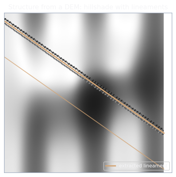
• Hillshade (illuminate the DEM from a low sun angle) makes lineaments, scarps, and fold traces pop. Rotate the illumination azimuth, because a single azimuth hides structures parallel to the light.
• Slope and curvature separate steep fault scarps and drainage incision from smooth interfluves; plan and profile curvature help segment landforms.
• Drainage and lineaments carry structural information: rivers often follow faults and lithological contacts, and automated lineament extraction (edge detection on hillshade and curvature, then vectorising) gives a first structural map to check against geology.

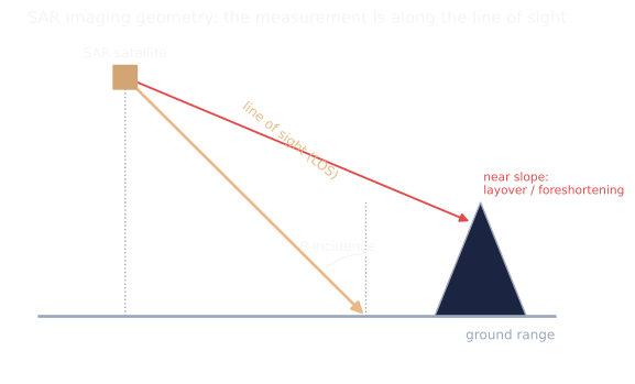
Copernicus GLO-30 (global, 30 m, open, from TanDEM-X 2011 to 2015) is the default DEM; SRTM and, where available, lidar are alternatives. SAR adds two things: amplitude images light one side of terrain strongly (slopes facing the sensor), which enhances some lineaments and hides others, and the same geometry that helps also fools you, because layover and shadow (Module 3) can masquerade as structure. Always cross-check a SAR-derived lineament against the DEM and the opposite look direction.

Machine learning enters as geomorphometry: classify landforms or segment terrain from DEM derivatives (a random forest on slope, curvature, roughness, and openness, or a CNN on the DEM), exactly the Module 4 and Module 7 machinery applied to elevation rather than reflectance.

Lesson 2: InSAR from the ground up for geoscientists

Interferometric SAR uses the phase of two SAR acquisitions (Single Look Complex, not GRD) over the same area. The phase difference, the interferogram, encodes any change in the sensor-to-ground distance between the two dates:

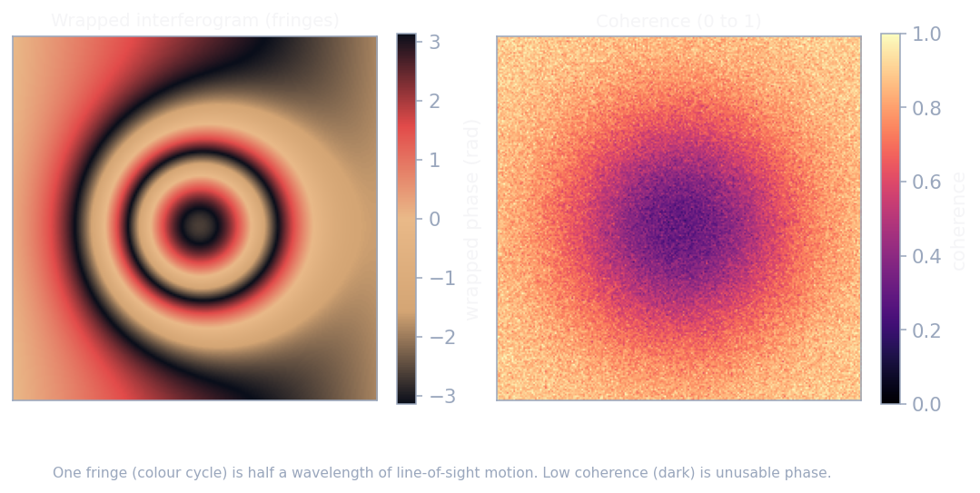
• Interferogram formation: coregister two SLCs, multiply one by the complex conjugate of the other, and you get interference fringes. Each full colour cycle (fringe) is half a wavelength of line-of-sight motion (about 2.8 cm for C-band Sentinel-1).
• Coherence measures how correlated the two acquisitions are, from 0 to 1. Vegetation, water, and long time gaps decorrelate (low coherence, unusable phase); bare rock, cities, and short intervals stay coherent. Coherence is both a mask and a signal, as you saw in Module 9.
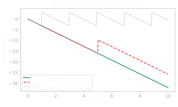
• Phase unwrapping turns the wrapped fringes (which only run 0 to 2 pi) into continuous displacement. Unwrapping errors, where the algorithm jumps a whole cycle, are a leading cause of wrong deformation maps.
• Error sources you must respect: the atmosphere (tropospheric delay adds phase that mimics deformation, especially over topography), residual DEM error, orbital ramps (long-wavelength tilts), and decorrelation. A single interferogram cannot separate a slow deformation signal from atmosphere; that is why you build a time series.

Lesson 3: PS, SBAS, and building a time series

One interferogram is noisy; a stack is a measurement. Two classic strategies turn a stack into a velocity:

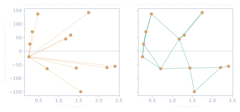
• Persistent Scatterer (PS) tracks individual pixels that stay bright and coherent over the whole stack (rock outcrops, buildings, infrastructure). It excels in cities and on engineered structures and gives point velocities with millimetre precision.
• Small Baseline Subset (SBAS) forms many interferograms between temporally and spatially close pairs, keeps distributed targets, and inverts the network for a displacement time series. It works better over more natural terrain.

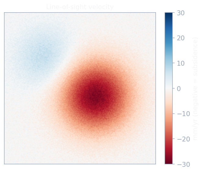
In practice you will use MintPy (the current open time-series stack) on top of HyP3 burst interferograms, which is the workflow this module's lab follows. The output is a line-of-sight velocity map and a per-pixel time series, plus the estimated errors. Remember the LOS caveat: InSAR measures motion along the radar line of sight, not vertical; converting to vertical requires an assumption (often "motion is vertical") or combining ascending and descending tracks.

Lesson 4: Earthquakes, volcanoes, and faulting

• Earthquakes produce coseismic deformation: a single interferogram spanning the event shows the surface displacement field, from which the fault geometry and slip can be inverted (an inverse problem: find the fault plane and slip that best reproduce the observed fringes). You do not need to master slip inversion here, but you should be able to read a coseismic interferogram and say where the fault is.
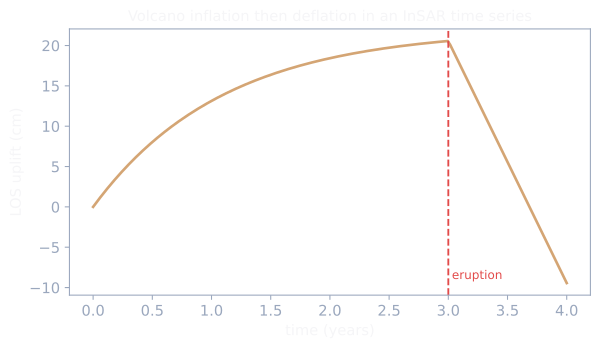
• Volcanoes inflate and deflate as magma moves, often months before an eruption, so InSAR time series over volcanoes are a monitoring tool. Complementary signals include SO2 (TROPOMI on Sentinel-5P) and thermal anomalies and lava mapping (Landsat and ASTER TIR, VIIRS). Machine learning now scans global InSAR archives for unrest automatically.

• Ready-made products save you processing: the ARIA project and the COMET LiCSAR archive publish standard interferograms and, via LiCSBAS, time series for much of the world's tectonic and volcanic terrain. Use these before you process your own when they cover your target.

Lesson 5: Landslides and subsidence

• Landslides: map inventories from optical and SAR change (Module 6), model susceptibility with ML (Module 9.6 does this with an area-of-applicability check), and detect slow-moving landslides directly with InSAR, where a coherent hillslope creeps a few centimetres a year.
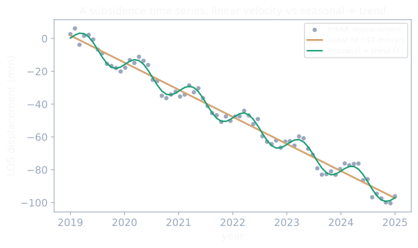
• Subsidence is the workhorse application and the subject of this module's lab. Groundwater extraction, oil and gas withdrawal, mining, and sediment compaction all cause the ground to sink, sometimes tens of centimetres a year. Two points matter for interpretation. First, coastal subsidence often exceeds sea-level rise, so relative sea-level change at a city is the sum of both; a place like Lagos or the Niger Delta can be losing elevation from compaction and extraction faster than the ocean is rising, which connects directly to infrastructure and pipeline risk in the PipelineWatch-NG setting. Second, subsidence over aquifers is often seasonal (elastic rebound when recharge returns) on top of a long-term inelastic trend, so a linear velocity alone can mislead.

Lesson 6: The wider geodesy toolkit, and a planetary coda

InSAR is one instrument among several, and interviews probe whether you know the trade-offs:

• GNSS gives sparse but highly accurate three-component displacement at fixed stations; it anchors and validates InSAR, which is dense but relative and one-dimensional.
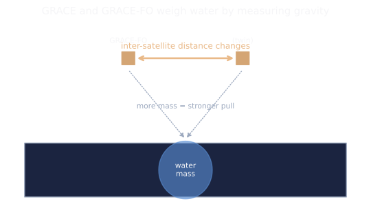
• GRACE and GRACE-FO weigh water by measuring tiny changes in Earth's gravity field from the distance between two satellites. They resolve total water storage (groundwater plus soil moisture plus surface water plus ice) at coarse scale (a few hundred kilometres), which is why GRACE is the tool for basin-scale groundwater depletion but useless for a single well field. GRACE-FO has flown since 2018; the GRACE-C continuity mission is planned for later this decade.

• Satellite gravity and magnetics (the GOCE gravity model, the EMAG2 magnetic anomaly grid, the WGM2012 gravity model) map deep and broad structure, crustal boundaries, and basins, at resolutions far coarser than airborne surveys (Module 9.6 uses airborne magnetics and gravity for exploration). They constrain the big picture, not the local target.

A short planetary coda: the same toolkit travels. DEMs, hillshade structural mapping, spectral mineralogy, and even radar work on Mars and the Moon (for example CTX and HiRISE terrain, CRISM spectra), and planetary geology roles use exactly these skills.

Guided lab (about 9 hours): an InSAR deformation time series

You will build a line-of-sight deformation time series over a real target, produce a velocity map, and interpret it honestly. A starter notebook notebooks/12_insar_deformation.ipynb scaffolds the HyP3 ordering and the MintPy call so you are not staring at a blank cell; you write the analysis and the interpretation.

Step 1: Choose a target and pull the DEM

Pick one of three, based on what you can defend in an interview:

1. A subsiding city or aquifer (for example Lagos or the Niger Delta, tying to infrastructure and pipeline risk; or a well-studied aquifer such as a Central Valley or Central Mexico site).
2. An active mine or tailings storage facility, where geotechnical teams monitor wall and dam deformation.
3. A volcano with documented unrest and good Sentinel-1 coverage.

Pull the Copernicus GLO-30 DEM over your area of interest (open, on AWS, Planetary Computer, or OpenTopography). Make a hillshade and note the main structures, so you can later separate real deformation from topographic artefacts.

Step 2: Order burst interferograms and run MintPy

Submit an ASF HyP3 INSAR_ISCE_BURST job (or INSAR_ISCE_MULTI_BURST for a wider area) for a short-baseline network of Sentinel-1 pairs over your target, using the hyp3_sdk Python package. When the products are ready, prepare them for MintPy (mintpy.prep_hyp3) and run the small-baseline time-series workflow (smallbaselineApp.py). This produces a line-of-sight velocity and a per-date displacement time series. Follow the ASF MintPy recipe book for the exact current commands, since the CLI evolves between releases.

If HyP3 processing is more than you want to run, use a ready-made COMET LiCSAR frame over your target and process it with LiCSBAS, or, only if your target is in North America, download an OPERA DISP-S1 product directly. State which route you took and why.

Step 3 (core): analyse the time series with tested helpers

Whatever route produced the stack, the analysis is the same and is where the learning is. Build insar_geo.py:

"""insar_geo.py: geoscience InSAR deformation helpers (pure, testable)."""
import numpy as np


def velocity_fit(times_years, disp):
    """Least-squares linear velocity from a displacement time series.

    times_years: decimal years; disp: displacement (mm). NaN samples are ignored.
    Returns (slope, intercept); slope is the velocity in mm per year.
    """
    t = np.asarray(times_years, float)
    d = np.asarray(disp, float)
    m = ~(np.isnan(t) | np.isnan(d))
    if m.sum() < 2:
        return float("nan"), float("nan")
    a = np.vstack([t[m], np.ones(m.sum())]).T
    slope, intercept = np.linalg.lstsq(a, d[m], rcond=None)[0]
    return float(slope), float(intercept)


def fit_r2(times_years, disp, slope, intercept):
    """R-squared of a linear velocity fit; a simple time-series quality score."""
    t = np.asarray(times_years, float)
    d = np.asarray(disp, float)
    m = ~(np.isnan(t) | np.isnan(d))
    if m.sum() < 2:
        return float("nan")
    pred = slope * t[m] + intercept
    ss_res = float(np.sum((d[m] - pred) ** 2))
    ss_tot = float(np.sum((d[m] - d[m].mean()) ** 2))
    return 1.0 if ss_tot == 0 else 1.0 - ss_res / ss_tot


def remove_planar_ramp(field):
    """Fit and subtract a planar ramp (a*x + b*y + c) from a 2D array.

    A crude orbital or long-wavelength atmospheric correction for an unwrapped
    interferogram or a velocity field. NaN pixels are ignored in the fit.
    """
    z = np.asarray(field, float)
    ny, nx = z.shape
    yy, xx = np.mgrid[0:ny, 0:nx]
    m = ~np.isnan(z)
    a = np.vstack([xx[m], yy[m], np.ones(m.sum())]).T
    coef, *_ = np.linalg.lstsq(a, z[m], rcond=None)
    ramp = coef[0] * xx + coef[1] * yy + coef[2]
    return z - ramp


def los_to_vertical(los, incidence_deg):
    """Convert line-of-sight to vertical, assuming purely vertical motion.

    vertical = LOS / cos(incidence). Valid where horizontal motion is negligible
    (subsidence and many volcanic and aquifer cases); state the assumption.
    """
    return np.asarray(los, float) / np.cos(np.deg2rad(np.asarray(incidence_deg, float)))


def classify_velocity(vel, subsidence_thresh=-10.0, uplift_thresh=10.0, nodata_code=255):
    """Classify a velocity array (mm/yr) into 0 stable, 1 subsidence, 2 uplift.

    Negative velocity is subsidence (moving away from a descending-track sensor or
    downward after LOS-to-vertical). NaN pixels map to nodata_code, never to a class.
    """
    v = np.asarray(vel, float)
    out = np.zeros(v.shape, dtype="uint8")
    out = np.where(v < subsidence_thresh, 1, out)
    out = np.where(v > uplift_thresh, 2, out)
    out = np.where(np.isnan(v), nodata_code, out).astype("uint8")
    return out

# tests/test_insar_geo.py
import numpy as np
from insar_geo import (
    classify_velocity,
    fit_r2,
    los_to_vertical,
    remove_planar_ramp,
    velocity_fit,
)


def test_velocity_fit_recovers_rate():
    rng = np.random.default_rng(0)
    t = np.linspace(2019.0, 2025.0, 60)
    true_rate = -18.0  # mm/yr subsidence
    d = true_rate * (t - t[0]) + 3.0 + rng.normal(0, 2.0, t.size)
    slope, _ = velocity_fit(t, d)
    assert abs(slope - true_rate) < 1.0


def test_velocity_fit_ignores_nan_and_needs_two():
    t = np.array([2020.0, 2021.0, np.nan])
    d = np.array([0.0, -10.0, 5.0])
    slope, _ = velocity_fit(t, d)
    assert abs(slope - (-10.0)) < 1e-9
    assert np.isnan(velocity_fit([2020.0], [1.0])[0])


def test_fit_r2_perfect_line():
    t = np.array([0.0, 1.0, 2.0, 3.0])
    d = 2.0 * t + 1.0
    assert abs(fit_r2(t, d, 2.0, 1.0) - 1.0) < 1e-12


def test_remove_planar_ramp_leaves_signal():
    ny, nx = 20, 25
    yy, xx = np.mgrid[0:ny, 0:nx]
    signal = np.zeros((ny, nx))
    signal[8:12, 10:14] = 5.0            # a localised deformation bump
    ramp = 2.0 * xx - 1.5 * yy + 7.0
    deramped = remove_planar_ramp(ramp + signal)
    # the planar ramp is removed (corner near zero) and the local signal survives
    assert abs(deramped[0, 0]) < 0.5
    assert deramped[8:12, 10:14].max() > 4.0


def test_los_to_vertical_known_values():
    assert abs(los_to_vertical(1.0, 0.0) - 1.0) < 1e-12
    assert abs(los_to_vertical(1.0, 60.0) - 2.0) < 1e-9


def test_classify_velocity_bands_and_nodata():
    vel = np.array([-20.0, 0.0, 25.0, np.nan])
    assert list(classify_velocity(vel)) == [1, 0, 2, 255]

Fit a velocity at a few representative points, deramp your velocity field, convert a subsidence signal to vertical with the track incidence, and classify the map into stable, subsiding, and uplifting. The tests encode the physics you must not get wrong: a linear fit recovers a known rate, a planar ramp is removable while a localised signal survives, LOS becomes vertical through the incidence angle, and NaN never silently becomes a class.

Step 4 (stretch, optional): validate and separate signals

Optional but strong: validate your InSAR velocity against a nearby GNSS station (or a published rate), and separate a seasonal (elastic) component from the long-term trend by fitting a trend-plus-annual model rather than a straight line. Mark this optional so the module stays near 14 hours without it.

Step 5: Write-up and commit

A short note, "Deformation at [target], [dates]," with the velocity map, one or two point time series, the LOS-to-vertical note, the error sources you considered, and an honest statement of what you can and cannot conclude. Commit insar_geo.py, its tests, and the notebook.

git add src/eo_portfolio/insar_geo.py tests/test_insar_geo.py notebooks/12_insar_deformation.ipynb
git commit -m "Module 9.5: InSAR deformation time series with tested helpers and a geohazard note"
git push

Checkpoint

Multiple choice (answers below).

1. One Sentinel-1 interferogram over a slowly subsiding city shows fringes that follow the topography closely. The most likely cause is: (a) real deformation exactly matching terrain; (b) tropospheric atmospheric delay correlated with elevation; (c) an unwrapping error; (d) DEM error only.
2. You want point-precise velocities on buildings and infrastructure in a dense city. You choose: (a) SBAS; (b) Persistent Scatterer; (c) a single interferogram; (d) GRACE.
3. InSAR measures: (a) vertical displacement directly; (b) three-component displacement; (c) displacement along the radar line of sight; (d) total water storage.
4. GRACE-FO is the right tool to: (a) map subsidence of a single well field at 30 m; (b) estimate basin-scale groundwater storage change; (c) invert a fault plane; (d) detect a slow-moving landslide.
5. To convert a line-of-sight subsidence rate to a vertical rate assuming vertical motion, you: (a) multiply by cos(incidence); (b) divide by cos(incidence); (c) divide by sin(incidence); (d) leave it unchanged.

Short answer (answers below).

1. Why can a single interferogram not separate slow deformation from atmosphere, and what fixes it?
2. Why is coherence both a mask and a signal?

Interview-style questions (practice out loud).

• Walk me through building a subsidence velocity map from Sentinel-1, and the three error sources you would worry about most.
• When would you use PS over SBAS, and why?
• A coastal city shows 3 cm/yr of relative sea-level rise. How do you use InSAR and tide-gauge or GNSS data to attribute it between subsidence and ocean rise?
• Your velocity map correlates with topography. How do you tell atmosphere from real deformation?
• When is GRACE the right instrument, and when is it useless?

Answers. (1) b: atmospheric delay is correlated with elevation and is the classic topography-correlated artefact; a time series or a weather-model correction separates it from deformation.
(2) b: PS tracks stable point scatterers such as buildings with millimetre precision.
(3) c: InSAR is one-dimensional along the line of sight; vertical needs an assumption or ascending-plus-descending tracks.
(4) b: GRACE and GRACE-FO resolve total water storage at a few hundred kilometres, ideal for basin groundwater, useless at field scale.
(5) b: vertical equals LOS divided by cos(incidence) under the vertical-motion assumption.
(6) A single interferogram mixes deformation, atmosphere, DEM error, and orbital ramp in one phase field, and atmosphere can mimic a deformation gradient; stacking many acquisitions into a time series (PS or SBAS) averages down the random atmosphere and isolates the persistent deformation.
(7) Low coherence marks pixels whose phase is unusable (vegetation, water, long gaps), so it masks; the pattern and loss of coherence itself also indicates change (clearing, flooding, construction), so it carries signal.

Deliverable

A tested insar_geo.py (velocity fit, R-squared, planar deramp, LOS-to-vertical, velocity classification), an InSAR deformation time series over your chosen target with a line-of-sight velocity map and at least one point time series, an honest note on error sources and the LOS-to-vertical assumption, and, optionally, a GNSS validation and a seasonal-plus-trend separation. This is the first half of the optional Geology and Geophysics elective and a portfolio piece few applicants have.

What a hiring manager sees

Deformation InSAR is a scarce, screened skill. Showing that you built a real velocity map, that you know it is line-of-sight and not vertical, that you can name and reason about atmosphere, unwrapping, and decorrelation, and that you interpret cautiously (seasonal versus inelastic, subsidence versus sea-level rise) marks you as someone a geodesy, volcano, insurance-geohazard, or mine-geotechnical team can trust. Referencing the current product landscape correctly (HyP3 burst InSAR, MintPy, COMET LiCSAR and LiCSBAS, OPERA DISP-S1 for North America, NISAR as it matures) signals you track the field, which is exactly what these employers want.

Currency note

Verified 22 August 2026. Copernicus DEM GLO-30 is open (TanDEM-X 2011 to 2015), available via AWS, Microsoft Planetary Computer, and OpenTopography. Sentinel-1 InSAR uses SLC data; Sentinel-1A ended operations in late June 2026, with Sentinel-1C and Sentinel-1D operational, so confirm which satellites cover your dates and note that a consistent InSAR stack should not straddle a satellite change without care. ASF HyP3 (version 10.17.x, with a credit system) offers on-demand INSAR_ISCE_BURST (single burst pair) and INSAR_ISCE_MULTI_BURST jobs via ASF Vertex, the HyP3 API, and hyp3_sdk; MintPy (1.6.4) processes the resulting stack, and the ASF OpenSARlab MintPy recipe book documents the current commands. COMET LiCSAR and LiCSBAS provide standard interferograms and time series for much of the tectonic and volcanic world. OPERA DISP-S1 (validated Version 1) covers North America only (the United States, territories within 200 km, Canada, and Central America to Panama, from mid-2016), so it is not a route over Nigeria, Australia, or most volcanoes. NISAR (NASA and ISRO) launched 30 July 2025; provisional L-band products are public from acquisitions since 17 June 2026, with validated products expected around Q4 2026. GRACE-FO has operated since 2018 and monitors total water storage; the GRACE-C continuity mission is planned for later this decade (around 2028). TROPOMI on Sentinel-5P provides SO2 for volcanoes. Confirm all product versions, coverage, and CLI options at study time, and pin your Python versions in the Module 0.1 environment file (insar_geo uses only NumPy).

Figures this module needs

1. InSAR imaging geometry and the line-of-sight vector, showing why the measurement is one-dimensional.
2. An interferogram and its coherence map, side by side, with fringes labelled as half-wavelength cycles.
3. A schematic contrasting Persistent Scatterer and Small Baseline Subset networks.
4. A subsidence line-of-sight velocity map over a city, with a colour bar in mm/yr.
5. A cartoon of an unwrapping error (a whole-cycle jump) versus true deformation.
6. A point time series with a linear velocity fit and a seasonal-plus-trend fit overlaid.
7. The GRACE mass-change concept: two satellites and the distance change that weighs water.
8. A hillshade with extracted lineaments overlaid, illustrating structure from a DEM.
9. A volcano inflation time series next to an SO2 or thermal snapshot.