Module 9: SAR Deep Learning, InSAR, and NISAR

Phase: III, Deep learning
Level: Advanced
Estimated time: ~12 hours (about 5 h concepts, 6 h lab, 1 h write-up)
Prerequisites: Modules 3 (SAR), 6 (SAR change), 7 (segmentation), 8.
Portfolio thread: a coherence-augmented change detector, a SAR flood model, and a NISAR-versus-Sentinel-1 note, a timely and rare portfolio piece. Closes Phase III.

Why this module

NISAR, the NASA-ISRO L-band and S-band radar mission, is now returning public data, and almost nobody on the job market has worked with it yet. Coherence, polarimetry, and SAR-specific deep learning are the differentiators for roles at SAR vendors and hazard-monitoring teams, and they are where general computer-vision skills stop being enough. This module takes you past amplitude-only SAR into the phase and polarization information that make radar uniquely powerful, and puts a genuinely current, scarce skill (hands-on NISAR) in your portfolio.

Learning outcomes

After this module you can:

1. Explain polarimetry and the Pauli decomposition intuition, and interferometry (interferogram, coherence, unwrapping).
2. Use coherence as a change and disturbance signal and add it to a detector.
3. Describe InSAR displacement time series (MintPy, SBAS, persistent scatterers) at a working-vocabulary level.
4. Train a SAR deep-learning model for flood segmentation and know the dark-vessel detection task.
5. Access NISAR L-band GCOV data and compare it to Sentinel-1 C-band.
6. Produce a coherence-augmented change detector, a SAR flood model, and a NISAR comparison note.

Concept lessons (about 5 hours)

Lesson 1: Polarimetry

Radar can transmit and receive in different polarizations, and fully polarimetric data (HH, HV, VH, VV) captures how a surface changes the polarization of the signal, which encodes its structure. The Pauli decomposition is the standard intuition: it splits the signal into surface scattering (HH plus VV), double-bounce (HH minus VV), and volume scattering (the cross-polarized term), which map to bare ground, buildings and flooded vegetation, and canopy respectively. Polarimetric features feed classification and are richer than the dual-pol VV and VH you used earlier.

Lesson 2: Interferometry and coherence

Two Single Look Complex acquisitions of the same place carry phase. Their phase difference is an interferogram, and after unwrapping it measures ground displacement toward or away from the sensor at centimeter or millimeter scale, which is how subsidence, landslides, and volcanic inflation are monitored. Alongside the phase, the correlation between the two acquisitions is the coherence, a number from 0 to 1: high coherence means a stable surface, and a drop in coherence means the surface changed between passes. This is why interferometry needs SLC products (which keep phase), not GRD.

Lesson 3: Coherence as a change signal

Coherence loss is a powerful, complementary change detector. Where vegetation is cleared, a structure is built, or a flood arrives, the scatterers rearrange and coherence collapses, even when backscatter amplitude barely moves. Adding coherence as a feature to the amplitude-based change detector from Module 6 typically improves it, because the two signals fail in different situations. You will measure that gain directly.

Lesson 4: InSAR displacement time series

Stacking many interferograms yields a displacement time series. The two dominant methods are Small Baseline Subset (SBAS) and Persistent Scatterers, and the open tool MintPy processes stacks into deformation maps. You do not need to specialize to be employable, but you must know the vocabulary (baselines, unwrapping errors, atmospheric phase screen) and that analysis-ready displacement products now exist (for example OPERA DISP-S1), so you can speak to it and use it.

Lesson 5: SAR deep learning and NISAR

• SAR deep learning: flood segmentation (datasets such as SEN12-FLOOD and ETCI) reuses your Module 7 segmentation stack, with speckle-aware augmentation; and dark-vessel detection (xView3-SAR) is the canonical maritime SAR task. Interestingly, ImageNet-pretrained encoders still transfer reasonably to SAR despite the domain gap, a useful practical fact.
• NISAR: the new L-band and S-band mission images the globe every 12 days. Its L-band penetrates the canopy far better than Sentinel-1 C-band, so it complements your C-band work for biomass, disturbance under vegetation, and flood beneath canopy. The Geocoded Polarimetric Covariance (GCOV) product gives radiometrically terrain-corrected, geocoded backscatter ready for analysis. Getting hands on NISAR now, while the data is fresh and few people have used it, is a standout portfolio move.

Lesson 6: Maritime domain awareness, ships and dark vessels

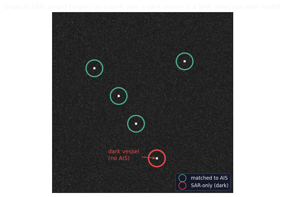
On open water SAR is close to ideal. Calm sea is smooth relative to the wavelength, so it scatters the pulse away and looks dark (the roughness idea from Module 3), while a metal ship is a strong corner reflector and shows up as a bright point. That contrast makes ship detection a classic SAR task, handled for decades with constant-false-alarm-rate (CFAR) detectors and now with deep learning.

The commercially valuable version is dark-vessel detection. Ships are meant to broadcast identity and position over AIS, but some switch it off to hide illegal fishing, sanctions evasion, or illicit ship-to-ship oil transfers. A vessel SAR sees but AIS does not report is "dark." The workflow: detect every vessel in the SAR scene, match detections to AIS tracks, and flag the unmatched ones. The canonical open dataset is xView3-SAR (nearly 1,000 Sentinel-1 scenes, over 220,000 labelled dark-vessel instances, built by matching global AIS to SAR), which plugs straight into your Module 7 and 9 detection stack.

This is a live market that maps to specific employers:

• ICEYE operates the largest X-band SAR constellation and sells a Dark Vessel Detection product that fuses its SAR with AIS for persistent maritime monitoring, and it also does oil-spill monitoring.
• Ursa Space Systems runs a virtual SAR constellation (aggregating many providers, tens of millions of SAR images) and fuses AIS with SAR detections for vessel analytics, alongside its global oil-storage inventory product (Module 9.6).
• Capella and Umbra provide very high-resolution SAR tasking to confirm and classify a specific vessel.
• Planet is optical, not SAR, but its daily PlanetScope and taskable SkySat imagery are used alongside SAR to visually confirm and identify a vessel once radar has found it, when it is daylit and cloud-free.

Being able to describe that pipeline (SAR detection, AIS fusion, optical confirmation) makes you directly relevant to maritime-security and SAR-analytics teams. The same "bright target on dark water" physics inverts for oil: an oil slick damps the waves and appears dark, which Module 9.6 covers.

Guided lab (about 6 hours): coherence, flood, and NISAR

Step 1: Coherence and a stronger change detector

Submit a HyP3 InSAR job for a pre-fire and post-fire Sentinel-1 pair and inspect the coherence loss over the burn. Then add coherence as a feature to your Module 6 change detector and measure the improvement.

"""insar.py: coherence and polarimetry helpers (pure, testable)."""
from __future__ import annotations
import numpy as np

def coherence(s1, s2, eps=1e-12):
    """Complex coherence magnitude between two SLC sample vectors (a window)."""
    s1 = np.asarray(s1); s2 = np.asarray(s2)
    num = np.abs(np.sum(s1 * np.conj(s2)))
    den = np.sqrt(np.sum(np.abs(s1) ** 2) * np.sum(np.abs(s2) ** 2)) + eps
    return float(num / den)

def coherence_change(coh, thresh=0.3):
    """Low coherence flags surface change between the two acquisitions."""
    return coh < thresh

def pauli_rgb(hh, hv, vv):
    """Pauli components (surface, double-bounce, volume) for RGB display.

    The full Pauli scattering vector carries a 1/sqrt(2) factor; it is dropped here
    because it only rescales all three channels equally and does not change the RGB
    appearance. Keep it if you need physically normalized components.
    """
    return (np.abs(hh + vv), np.abs(hh - vv), 2.0 * np.abs(hv))

# tests/test_insar.py
import numpy as np
from eo_portfolio.insar import coherence, coherence_change, pauli_rgb

def test_coherence_identical_is_one():
    rng = np.random.default_rng(0)
    s = rng.normal(size=64) + 1j * rng.normal(size=64)
    assert coherence(s, s) > 0.999

def test_coherence_uncorrelated_is_low():
    rng = np.random.default_rng(0)
    a = rng.normal(size=4096) + 1j * rng.normal(size=4096)
    b = rng.normal(size=4096) + 1j * rng.normal(size=4096)
    assert coherence(a, b) < 0.1

def test_coherence_change_and_pauli():
    assert coherence_change(0.2) and not coherence_change(0.5)
    s, d, v = pauli_rgb(np.array(1 + 0j), np.array(0 + 0j), np.array(1 + 0j))
    assert abs(s - 2) < 1e-9 and abs(d) < 1e-9 and abs(v) < 1e-9

Step 2: A SAR flood model

Train a small flood-segmentation model on SEN12-FLOOD or ETCI using your Module 7 segmentation stack, with speckle-aware augmentation. Note how the skills transfer directly to water and oil-slick mapping.

Step 2b (optional stretch): dark-vessel detection

Using xView3-SAR, detect vessels in Sentinel-1 scenes with your Module 7 and 9 detection stack, then match detections to the provided AIS labels and flag the unmatched "dark" vessels. Report detection precision and recall and the dark-vessel rate. This is a directly marketable maritime-security portfolio piece.

Step 3: NISAR versus Sentinel-1

Download a NISAR L-band GCOV granule over a forested part of your AOI from ASF, and compare L-band HH and HV to Sentinel-1 C-band VV and VH for the same area and near-date. Describe what the longer L-band wavelength reveals that C-band does not (deeper canopy interaction, different sensitivity), with figures.

Step 4: Write-up and commit

A short comparison note, "NISAR L-band versus Sentinel-1 C-band over forest," plus the coherence-augmented detector result and the flood model. Commit insar.py, tests, notebooks, and the note.

git add src/eo_portfolio/insar.py tests/test_insar.py notebooks/11_coherence_flood_nisar.ipynb writeups/03_nisar_vs_s1.md
git commit -m "Module 9: coherence change, SAR flood model, NISAR vs S1 comparison"
git push

Checkpoint

Self-check (answers below).

1. Why does interferometry require SLC products rather than GRD?
2. What does a drop in coherence between two acquisitions indicate, and why does it complement amplitude change?
3. What does NISAR's L-band see over forest that Sentinel-1 C-band does not?
4. What is the Pauli decomposition, physically?

Interview-style questions (practice out loud).

• Explain coherence to a product manager in three sentences.
• How would you add InSAR coherence to an existing amplitude change detector, and what would you expect to gain?
• When would you reach for NISAR L-band over Sentinel-1, and what does that change for biomass or flood-under-canopy?
• How would you approach dark-vessel detection from SAR, and what makes it hard?
• A ship shows in your SAR scene but not in AIS. What does that mean, how do you confirm it, and which sensors and companies would you reach for?
• Why does an oil slick look dark in SAR while a ship looks bright?

Answers. (1) Interferometry uses the phase difference between two acquisitions, and only SLC products preserve phase; GRD is detected amplitude with phase discarded.
(2) Coherence loss means the surface scatterers rearranged (clearing, construction, flood), so it detects change even when amplitude barely moves, and because the two signals fail differently, combining them is stronger.
(3) L-band's longer wavelength penetrates deeper into the canopy to branches and trunks, so it senses structure and biomass and disturbance under vegetation that C-band, which saturates on the upper canopy, misses.
(4) It splits the polarimetric signal into surface scattering (HH plus VV), double-bounce (HH minus VV), and volume scattering (cross-pol), corresponding physically to bare ground, structures or flooded vegetation, and canopy.

Deliverable

A tested insar.py (coherence, coherence-change, Pauli), a coherence-augmented change detector showing the measured gain over Module 6, a SAR flood-segmentation model, and a NISAR-versus-Sentinel-1 comparison note with figures. This closes Phase III and gives you a portfolio piece almost no other applicant will have.

What a hiring manager sees

Coherence, polarimetry, and hands-on NISAR are exactly the differentiators SAR-vendor and hazard teams screen for, and they are rare on the market. A candidate who can add coherence to a detector and show the gain, train a SAR flood model, and speak credibly about L-band NISAR versus C-band Sentinel-1, with figures, stands out immediately in 2026. Maritime and SAR-analytics teams (ICEYE, Ursa Space, Capella, Umbra) additionally screen for dark-vessel detection: SAR ship detection fused with AIS, and knowing when to bring in high-cadence optical (Planet) to confirm a target. The NISAR comparison signals that you move with the field the moment new data lands.

Currency note

Verified August 2026. NISAR (NASA and ISRO) launched on 30 July 2025 and is operational with a 12-day repeat. Beta L-band products were released in February 2026, and fully calibrated provisional L-band products are now public for acquisitions since 17 June 2026 (public release began 20 July 2026), available from ASF via Earthdata Search, ASF Vertex, the ASF SearchAPI, and the asf_search package. The GCOV (Geocoded Polarimetric Covariance) product is radiometrically terrain-corrected, projected to UTM at 10 to 20 m. Confirm the current product versions and coverage before the lab, since NISAR products are actively maturing from beta to provisional to validated. HyP3 provides on-demand Sentinel-1 InSAR and coherence; OPERA DISP-S1 provides analysis-ready displacement; MintPy processes InSAR stacks. SEN12-FLOOD, ETCI, and xView3-SAR are the standard SAR deep-learning datasets. Pin versions in your Module 0.1 environment file.